Location
Location ANSS
The ANSS event ID is uw60575952 and the event page is at
https://earthquake.usgs.gov/earthquakes/eventpage/uw60575952/executive.
2013/08/20 18:41:30 47.366 -122.717 13.3 3.6 Washington
Focal Mechanism
 USGS/SLU Moment Tensor Solution
 ENS  2013/08/20 18:41:30:0  47.37 -122.72  13.3 3.6 Washington

 Stations used:
   IU.COR US.HAWA UW.DOSE UW.LEBA UW.PHIN UW.RADR UW.RATT
   UW.TOLT UW.WOLL

 Filtering commands used:
   cut a -30 a 140
   rtr
   taper w 0.1
   hp c 0.03 n 3
   lp c 0.06 n 3
   br c 0.12 0.25 n 4 p 2

 Best Fitting Double Couple
  Mo = 9.12e+20 dyne-cm
  Mw = 3.24
  Z  = 2 km
  Plane   Strike  Dip  Rake
   NP1      169    58   138
   NP2      285    55    40
  Principal Axes:
   Axis    Value   Plunge  Azimuth
    T   9.12e+20     51     135
    N   0.00e+00     39     319
    P  -9.12e+20      2     228

 Moment Tensor: (dyne-cm)
    Component   Value
       Mxx    -2.28e+20
       Mxy    -6.33e+20
       Mxz    -2.97e+20
       Myy    -3.23e+20
       Myz     3.35e+20
       Mzz     5.51e+20


                     ##------------
                 #####-----------------
              #######---------------------
             ########----------------------
           #########-------------------------
          ##########--------------------------
         ####-------###########----------------
        #----------#################------------
        -----------####################---------
       -------------######################-------
       -------------########################-----
       -------------##########################---
       -------------###########################--
        -------------############   ############
        -------------############ T ############
         -------------###########   ###########
          -------------#######################
           -   ---------#####################
             P ----------##################
               -----------################
                 -----------###########
                     ---------#####


 Global CMT Convention Moment Tensor:
      R          T          P
  5.51e+20  -2.97e+20  -3.35e+20
 -2.97e+20  -2.28e+20   6.33e+20
 -3.35e+20   6.33e+20  -3.23e+20


Details of the solution is found at

http://www.eas.slu.edu/eqc/eqc_mt/MECH.NA/20130820184130/index.html
|
Preferred Solution
The preferred solution from an analysis of the surface-wave spectral amplitude radiation pattern, waveform inversion or first motion observations is
      STK = 285
      DIP = 55
     RAKE = 40
       MW = 3.24
       HS = 2.0
The NDK file is 20130820184130.ndk
The waveform inversion is preferred.
Moment Tensor Comparison
The following compares this source inversion to those provided by others. The purpose is to look for major differences and also to note slight differences that might be inherent to the processing procedure. For completeness the USGS/SLU solution is repeated from above.
| SLU |
USGSMT |
 USGS/SLU Moment Tensor Solution
 ENS  2013/08/20 18:41:30:0  47.37 -122.72  13.3 3.6 Washington

 Stations used:
   IU.COR US.HAWA UW.DOSE UW.LEBA UW.PHIN UW.RADR UW.RATT
   UW.TOLT UW.WOLL

 Filtering commands used:
   cut a -30 a 140
   rtr
   taper w 0.1
   hp c 0.03 n 3
   lp c 0.06 n 3
   br c 0.12 0.25 n 4 p 2

 Best Fitting Double Couple
  Mo = 9.12e+20 dyne-cm
  Mw = 3.24
  Z  = 2 km
  Plane   Strike  Dip  Rake
   NP1      169    58   138
   NP2      285    55    40
  Principal Axes:
   Axis    Value   Plunge  Azimuth
    T   9.12e+20     51     135
    N   0.00e+00     39     319
    P  -9.12e+20      2     228

 Moment Tensor: (dyne-cm)
    Component   Value
       Mxx    -2.28e+20
       Mxy    -6.33e+20
       Mxz    -2.97e+20
       Myy    -3.23e+20
       Myz     3.35e+20
       Mzz     5.51e+20


                     ##------------
                 #####-----------------
              #######---------------------
             ########----------------------
           #########-------------------------
          ##########--------------------------
         ####-------###########----------------
        #----------#################------------
        -----------####################---------
       -------------######################-------
       -------------########################-----
       -------------##########################---
       -------------###########################--
        -------------############   ############
        -------------############ T ############
         -------------###########   ###########
          -------------#######################
           -   ---------#####################
             P ----------##################
               -----------################
                 -----------###########
                     ---------#####


 Global CMT Convention Moment Tensor:
      R          T          P
  5.51e+20  -2.97e+20  -3.35e+20
 -2.97e+20  -2.28e+20   6.33e+20
 -3.35e+20   6.33e+20  -3.23e+20


Details of the solution is found at

http://www.eas.slu.edu/eqc/eqc_mt/MECH.NA/20130820184130/index.html
|
|
Context
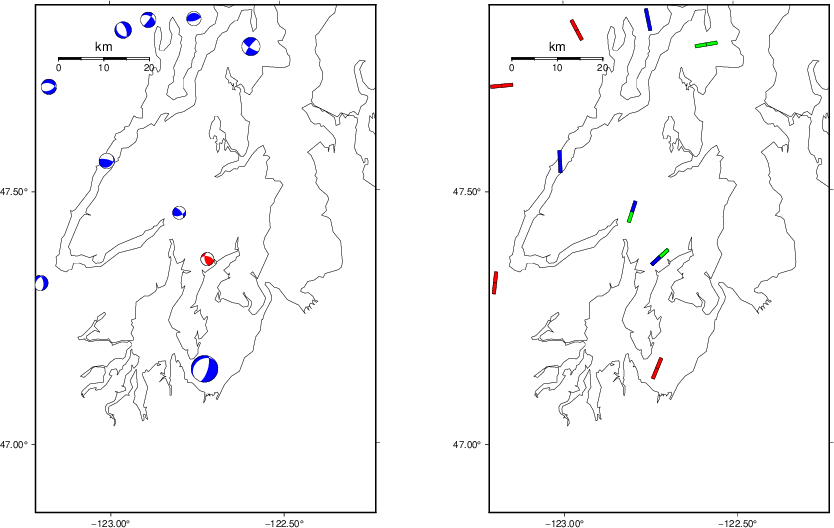
The left panel of the next figure presents the focal mechanism for this earthquake (red) in the context of other nearby events (blue) in the SLU Moment Tensor Catalog. The right panel shows the inferred direction of maximum compressive stress and the type of faulting (green is strike-slip, red is normal, blue is thrust; oblique is shown by a combination of colors). Thus context plot is useful for assessing the appropriateness of the moment tensor of this event.
Waveform Inversion using wvfgrd96
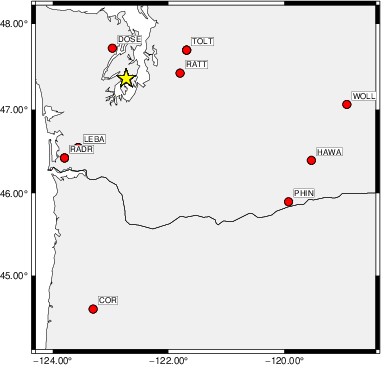
The focal mechanism was determined using broadband seismic waveforms. The location of the event (star) and the
stations used for (red) the waveform inversion are shown in the next figure.
|
|
Location of broadband stations used for waveform inversion
|
The program wvfgrd96 was used with good traces observed at short distance to determine the focal mechanism, depth and seismic moment. This technique requires a high quality signal and well determined velocity model for the Green's functions. To the extent that these are the quality data, this type of mechanism should be preferred over the radiation pattern technique which requires the separate step of defining the pressure and tension quadrants and the correct strike.
The observed and predicted traces are filtered using the following gsac commands:
cut a -30 a 140
rtr
taper w 0.1
hp c 0.03 n 3
lp c 0.06 n 3
br c 0.12 0.25 n 4 p 2
The results of this grid search are as follow:
           DEPTH  STK   DIP  RAKE   MW    FIT
WVFGRD96    0.5   120    50    65   3.12 0.4897
WVFGRD96    1.0   285    55    35   3.16 0.4735
WVFGRD96    2.0   285    55    40   3.24 0.5535
WVFGRD96    3.0   285    55    35   3.30 0.5513
WVFGRD96    4.0   285    50    35   3.35 0.5241
WVFGRD96    5.0   280    45    25   3.37 0.4837
WVFGRD96    6.0   275    50     5   3.38 0.4562
WVFGRD96    7.0   275    65   -10   3.39 0.4570
WVFGRD96    8.0   130    65    85   3.40 0.4516
WVFGRD96    9.0   270    60   -20   3.42 0.4499
WVFGRD96   10.0   270    65   -25   3.42 0.4518
WVFGRD96   11.0   270    65   -25   3.43 0.4529
WVFGRD96   12.0   270    65   -25   3.43 0.4512
WVFGRD96   13.0   270    65   -25   3.43 0.4492
WVFGRD96   14.0    85    65   -45   3.42 0.4451
WVFGRD96   15.0    85    60   -40   3.43 0.4466
WVFGRD96   16.0    80    60   -50   3.43 0.4482
WVFGRD96   17.0   115    70   -40   3.42 0.4511
WVFGRD96   18.0   115    70   -45   3.41 0.4534
WVFGRD96   19.0   115    70   -45   3.41 0.4546
WVFGRD96   20.0   120    70   -45   3.41 0.4551
WVFGRD96   21.0   120    70   -50   3.41 0.4533
WVFGRD96   22.0   120    70   -50   3.42 0.4535
WVFGRD96   23.0   120    70   -50   3.43 0.4527
WVFGRD96   24.0    25    45   -35   3.44 0.4545
WVFGRD96   25.0    20    45   -40   3.46 0.4560
WVFGRD96   26.0    20    45   -40   3.47 0.4564
WVFGRD96   27.0    20    45   -40   3.48 0.4555
WVFGRD96   28.0    20    45   -40   3.49 0.4532
WVFGRD96   29.0    20    45   -40   3.50 0.4495
The best solution is
WVFGRD96 2.0 285 55 40 3.24 0.5535
The mechanism corresponding to the best fit is
|
|
Figure 1. Waveform inversion focal mechanism
|
The best fit as a function of depth is given in the following figure:
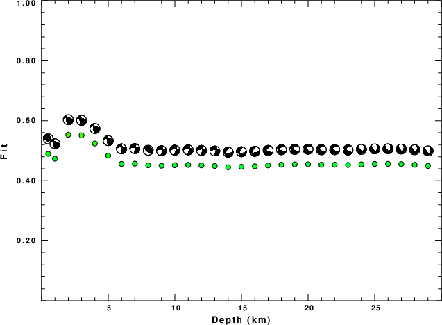
|
|
Figure 2. Depth sensitivity for waveform mechanism
|
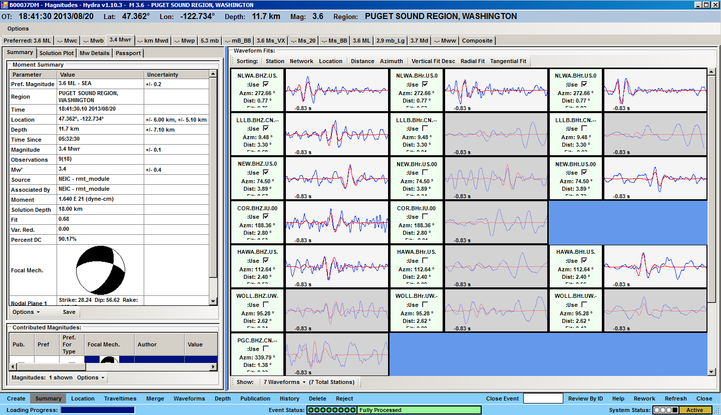
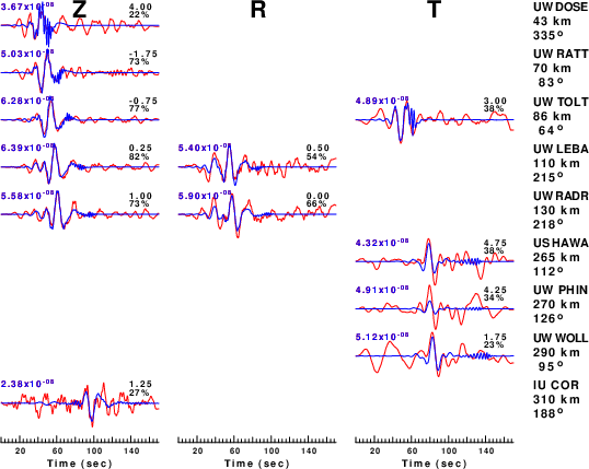
The comparison of the observed and predicted waveforms is given in the next figure. The red traces are the observed and the blue are the predicted.
Each observed-predicted component is plotted to the same scale and peak amplitudes are indicated by the numbers to the left of each trace. A pair of numbers is given in black at the right of each predicted traces. The upper number it the time shift required for maximum correlation between the observed and predicted traces. This time shift is required because the synthetics are not computed at exactly the same distance as the observed, the velocity model used in the predictions may not be perfect and the epicentral parameters may be be off.
A positive time shift indicates that the prediction is too fast and should be delayed to match the observed trace (shift to the right in this figure). A negative value indicates that the prediction is too slow. The lower number gives the percentage of variance reduction to characterize the individual goodness of fit (100% indicates a perfect fit).
The bandpass filter used in the processing and for the display was
cut a -30 a 140
rtr
taper w 0.1
hp c 0.03 n 3
lp c 0.06 n 3
br c 0.12 0.25 n 4 p 2
|
|
Figure 3. Waveform comparison for selected depth. Red: observed; Blue - predicted. The time shift with respect to the model prediction is indicated. The percent of fit is also indicated. The time scale is relative to the first trace sample.
|
|
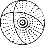
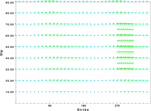
|
Focal mechanism sensitivity at the preferred depth. The red color indicates a very good fit to the waveforms.
Each solution is plotted as a vector at a given value of strike and dip with the angle of the vector representing the rake angle, measured, with respect to the upward vertical (N) in the figure.
|
A check on the assumed source location is possible by looking at the time shifts between the observed and predicted traces. The time shifts for waveform matching arise for several reasons:
- The origin time and epicentral distance are incorrect
- The velocity model used for the inversion is incorrect
- The velocity model used to define the P-arrival time is not the
same as the velocity model used for the waveform inversion
(assuming that the initial trace alignment is based on the
P arrival time)
Assuming only a mislocation, the time shifts are fit to a functional form:
Time_shift = A + B cos Azimuth + C Sin Azimuth
The time shifts for this inversion lead to the next figure:
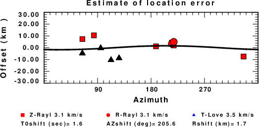
The derived shift in origin time and epicentral coordinates are given at the bottom of the figure.
Velocity Model
The WUS.model used for the waveform synthetic seismograms and for the surface wave eigenfunctions and dispersion is as follows
(The format is in the model96 format of Computer Programs in Seismology).
MODEL.01
Model after     8 iterations
ISOTROPIC
KGS
FLAT EARTH
1-D
CONSTANT VELOCITY
LINE08
LINE09
LINE10
LINE11
      H(KM)   VP(KM/S)   VS(KM/S) RHO(GM/CC)         QP         QS       ETAP       ETAS      FREFP      FREFS
     1.9000     3.4065     2.0089     2.2150  0.302E-02  0.679E-02   0.00       0.00       1.00       1.00
     6.1000     5.5445     3.2953     2.6089  0.349E-02  0.784E-02   0.00       0.00       1.00       1.00
    13.0000     6.2708     3.7396     2.7812  0.212E-02  0.476E-02   0.00       0.00       1.00       1.00
    19.0000     6.4075     3.7680     2.8223  0.111E-02  0.249E-02   0.00       0.00       1.00       1.00
     0.0000     7.9000     4.6200     3.2760  0.164E-10  0.370E-10   0.00       0.00       1.00       1.00
Last Changed Sat Apr 27 10:38:07 AM CDT 2024