Location
Location ANSS
The ANSS event ID is ak0139xclbxw and the event page is at
https://earthquake.usgs.gov/earthquakes/eventpage/ak0139xclbxw/executive.
2013/08/04 07:57:54 61.440 -149.861 36.7 3.8 Alaska
Focal Mechanism
 USGS/SLU Moment Tensor Solution
 ENS  2013/08/04 07:57:54:0  61.44 -149.86  36.7 3.8 Alaska

 Stations used:
   AK.FID AK.GHO AK.GLI AK.RC01 AK.SAW AK.SCM AK.SKN AK.SSN
   AK.SWD AT.PMR

 Filtering commands used:
   cut a -30 a 120
   rtr
   taper w 0.1
   hp c 0.02 n 3
   lp c 0.06 n 3

 Best Fitting Double Couple
  Mo = 1.02e+22 dyne-cm
  Mw = 3.94
  Z  = 48 km
  Plane   Strike  Dip  Rake
   NP1      220    70   -60
   NP2      341    36   -144
  Principal Axes:
   Axis    Value   Plunge  Azimuth
    T   1.02e+22     19     288
    N   0.00e+00     28      29
    P  -1.02e+22     55     168

 Moment Tensor: (dyne-cm)
    Component   Value
       Mxx    -2.38e+21
       Mxy    -1.97e+21
       Mxz     5.70e+21
       Myy     8.08e+21
       Myz    -4.08e+21
       Mzz    -5.70e+21


                     ##------------
                 ############----------
              ##################---------#
             ######################-#######
           ######################---#########
          #####################-------########
         ####################----------########
        ##   ##############-------------########
        ## T ############----------------#######
       ###   ###########-----------------########
       ###############--------------------#######
       ##############---------------------#######
       #############----------------------#######
        ###########-----------------------######
        ##########----------   -----------######
         ########----------- P -----------#####
          ######------------   ----------#####
           ####-------------------------#####
             ##-------------------------###
              #-----------------------####
                 --------------------##
                     --------------


 Global CMT Convention Moment Tensor:
      R          T          P
 -5.70e+21   5.70e+21   4.08e+21
  5.70e+21  -2.38e+21   1.97e+21
  4.08e+21   1.97e+21   8.08e+21


Details of the solution is found at

http://www.eas.slu.edu/eqc/eqc_mt/MECH.NA/20130804075754/index.html
|
Preferred Solution
The preferred solution from an analysis of the surface-wave spectral amplitude radiation pattern, waveform inversion or first motion observations is
      STK = 220
      DIP = 70
     RAKE = -60
       MW = 3.94
       HS = 48.0
The NDK file is 20130804075754.ndk
The waveform inversion is preferred.
Magnitudes
Given the availability of digital waveforms for determination of the moment tensor, this section documents the added processing leading to mLg, if appropriate to the region, and ML by application of the respective IASPEI formulae. As a research study, the linear distance term of the IASPEI formula
for ML is adjusted to remove a linear distance trend in residuals to give a regionally defined ML. The defined ML uses horizontal component recordings, but the same procedure is applied to the vertical components since there may be some interest in vertical component ground motions. Residual plots versus distance may indicate interesting features of ground motion scaling in some distance ranges. A residual plot of the regionalized magnitude is given as a function of distance and azimuth, since data sets may transcend different wave propagation provinces.
ML Magnitude
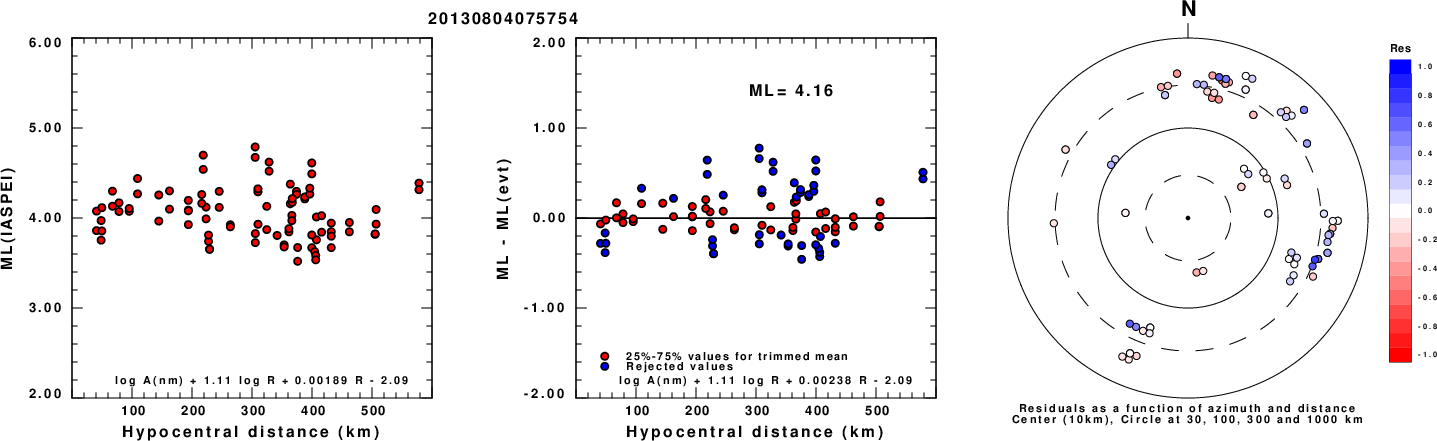
Left: ML computed using the IASPEI formula for Horizontal components. Center: ML residuals computed using a modified IASPEI formula that accounts for path specific attenuation; the values used for the trimmed mean are indicated. The ML relation used for each figure is given at the bottom of each plot.
Right: Residuals from new relation as a function of distance and azimuth.
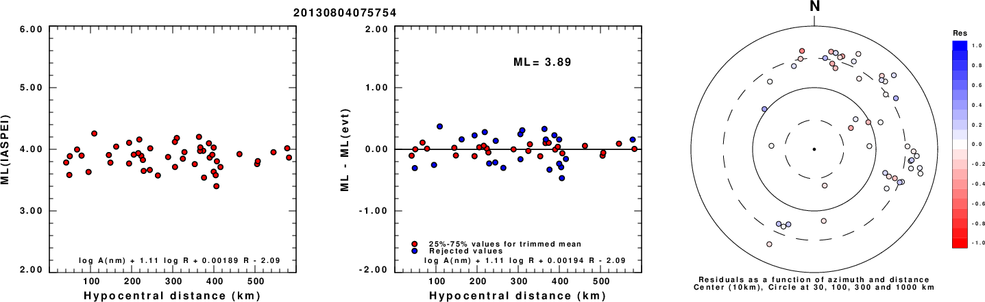
Left: ML computed using the IASPEI formula for Vertical components (research). Center: ML residuals computed using a modified IASPEI formula that accounts for path specific attenuation; the values used for the trimmed mean are indicated. The ML relation used for each figure is given at the bottom of each plot.
Right: Residuals from new relation as a function of distance and azimuth.
Context
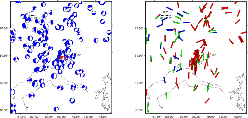
The left panel of the next figure presents the focal mechanism for this earthquake (red) in the context of other nearby events (blue) in the SLU Moment Tensor Catalog. The right panel shows the inferred direction of maximum compressive stress and the type of faulting (green is strike-slip, red is normal, blue is thrust; oblique is shown by a combination of colors). Thus context plot is useful for assessing the appropriateness of the moment tensor of this event.
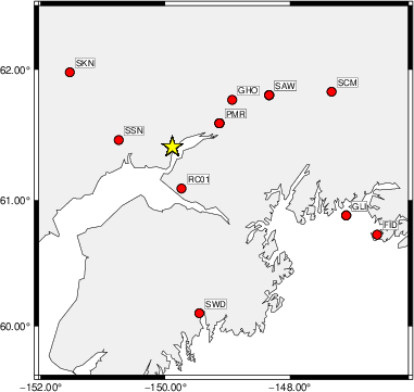
Waveform Inversion using wvfgrd96
The focal mechanism was determined using broadband seismic waveforms. The location of the event (star) and the
stations used for (red) the waveform inversion are shown in the next figure.
|
|
Location of broadband stations used for waveform inversion
|
The program wvfgrd96 was used with good traces observed at short distance to determine the focal mechanism, depth and seismic moment. This technique requires a high quality signal and well determined velocity model for the Green's functions. To the extent that these are the quality data, this type of mechanism should be preferred over the radiation pattern technique which requires the separate step of defining the pressure and tension quadrants and the correct strike.
The observed and predicted traces are filtered using the following gsac commands:
cut a -30 a 120
rtr
taper w 0.1
hp c 0.02 n 3
lp c 0.06 n 3
The results of this grid search are as follow:
           DEPTH  STK   DIP  RAKE   MW    FIT
WVFGRD96    0.5    25    45    95   3.22 0.2646
WVFGRD96    1.0   195    45    90   3.24 0.2639
WVFGRD96    2.0   195    45    85   3.37 0.3455
WVFGRD96    3.0   190    50    80   3.42 0.3495
WVFGRD96    4.0    15    45   -90   3.46 0.3490
WVFGRD96    5.0   225    80   -10   3.42 0.3568
WVFGRD96    6.0   230    80    -5   3.43 0.3698
WVFGRD96    7.0   240    70    -5   3.45 0.3841
WVFGRD96    8.0   240    70    -5   3.48 0.3995
WVFGRD96    9.0    70    60    30   3.52 0.4079
WVFGRD96   10.0    70    65    30   3.54 0.4211
WVFGRD96   11.0    70    65    30   3.55 0.4354
WVFGRD96   12.0    70    65    30   3.56 0.4482
WVFGRD96   13.0    70    65    30   3.57 0.4591
WVFGRD96   14.0    70    65    30   3.59 0.4689
WVFGRD96   15.0    75    65    25   3.60 0.4779
WVFGRD96   16.0    70    70    30   3.61 0.4864
WVFGRD96   17.0    70    70    25   3.62 0.4941
WVFGRD96   18.0    70    70    25   3.63 0.5017
WVFGRD96   19.0    70    70    25   3.64 0.5087
WVFGRD96   20.0    70    70    25   3.65 0.5149
WVFGRD96   21.0   230    70   -35   3.67 0.5248
WVFGRD96   22.0   230    70   -40   3.68 0.5381
WVFGRD96   23.0   230    70   -40   3.69 0.5510
WVFGRD96   24.0   230    70   -40   3.69 0.5626
WVFGRD96   25.0   230    70   -40   3.70 0.5735
WVFGRD96   26.0   230    70   -40   3.71 0.5841
WVFGRD96   27.0   230    70   -40   3.72 0.5927
WVFGRD96   28.0   230    70   -40   3.72 0.6011
WVFGRD96   29.0   230    70   -40   3.73 0.6077
WVFGRD96   30.0   230    75   -45   3.74 0.6139
WVFGRD96   31.0   230    75   -45   3.75 0.6221
WVFGRD96   32.0   230    75   -45   3.75 0.6282
WVFGRD96   33.0   225    70   -45   3.76 0.6350
WVFGRD96   34.0   225    70   -45   3.76 0.6400
WVFGRD96   35.0   225    70   -45   3.77 0.6465
WVFGRD96   36.0   225    70   -45   3.78 0.6519
WVFGRD96   37.0   225    70   -45   3.79 0.6571
WVFGRD96   38.0   225    70   -45   3.79 0.6608
WVFGRD96   39.0   220    70   -45   3.81 0.6654
WVFGRD96   40.0   225    70   -60   3.90 0.6622
WVFGRD96   41.0   225    70   -55   3.90 0.6680
WVFGRD96   42.0   225    70   -55   3.91 0.6723
WVFGRD96   43.0   220    70   -55   3.91 0.6768
WVFGRD96   44.0   220    70   -55   3.92 0.6795
WVFGRD96   45.0   220    70   -55   3.93 0.6821
WVFGRD96   46.0   220    70   -55   3.93 0.6832
WVFGRD96   47.0   220    70   -60   3.94 0.6838
WVFGRD96   48.0   220    70   -60   3.94 0.6840
WVFGRD96   49.0   220    70   -60   3.95 0.6833
WVFGRD96   50.0   220    70   -60   3.95 0.6823
WVFGRD96   51.0   220    70   -60   3.95 0.6802
WVFGRD96   52.0   220    70   -60   3.96 0.6782
WVFGRD96   53.0   220    70   -60   3.96 0.6753
WVFGRD96   54.0   220    70   -60   3.96 0.6726
WVFGRD96   55.0   220    70   -60   3.96 0.6693
WVFGRD96   56.0   220    70   -60   3.97 0.6651
WVFGRD96   57.0   220    70   -60   3.97 0.6616
WVFGRD96   58.0   220    70   -60   3.97 0.6563
WVFGRD96   59.0   215    70   -60   3.97 0.6534
WVFGRD96   60.0   215    70   -60   3.98 0.6491
WVFGRD96   61.0   215    70   -60   3.98 0.6452
WVFGRD96   62.0   215    70   -60   3.98 0.6407
WVFGRD96   63.0   215    70   -60   3.98 0.6363
WVFGRD96   64.0   215    70   -60   3.98 0.6329
WVFGRD96   65.0   215    70   -60   3.98 0.6282
WVFGRD96   66.0   215    70   -60   3.98 0.6239
WVFGRD96   67.0   215    70   -60   3.99 0.6205
WVFGRD96   68.0   215    70   -60   3.99 0.6153
WVFGRD96   69.0   215    70   -60   3.99 0.6115
WVFGRD96   70.0   215    70   -60   3.99 0.6073
WVFGRD96   71.0   215    70   -60   3.99 0.6022
WVFGRD96   72.0   215    70   -60   3.99 0.5988
WVFGRD96   73.0   215    70   -60   3.99 0.5944
WVFGRD96   74.0   215    70   -60   3.99 0.5894
WVFGRD96   75.0   215    70   -60   3.99 0.5861
WVFGRD96   76.0   215    75   -60   4.00 0.5818
WVFGRD96   77.0   215    75   -60   4.00 0.5786
WVFGRD96   78.0   215    75   -60   4.00 0.5755
WVFGRD96   79.0   215    75   -60   4.00 0.5730
WVFGRD96   80.0   215    75   -65   4.00 0.5697
WVFGRD96   81.0   215    75   -65   4.01 0.5665
WVFGRD96   82.0   215    75   -65   4.01 0.5644
WVFGRD96   83.0   215    75   -65   4.01 0.5612
WVFGRD96   84.0   215    75   -65   4.01 0.5580
WVFGRD96   85.0   215    75   -65   4.01 0.5555
WVFGRD96   86.0   215    75   -65   4.01 0.5532
WVFGRD96   87.0   215    75   -70   4.01 0.5495
WVFGRD96   88.0   215    80   -70   4.02 0.5476
WVFGRD96   89.0   215    80   -70   4.02 0.5458
WVFGRD96   90.0   215    80   -70   4.03 0.5443
WVFGRD96   91.0   215    80   -75   4.03 0.5415
WVFGRD96   92.0   215    80   -75   4.03 0.5409
WVFGRD96   93.0   215    80   -80   4.04 0.5389
WVFGRD96   94.0   215    80   -85   4.05 0.5373
WVFGRD96   95.0   215    80   -85   4.05 0.5357
WVFGRD96   96.0   215    80   -85   4.05 0.5346
WVFGRD96   97.0   215    80   -85   4.05 0.5329
WVFGRD96   98.0   215    80   -85   4.05 0.5308
WVFGRD96   99.0   215    80   -85   4.05 0.5292
WVFGRD96  100.0   215    80   -85   4.05 0.5273
WVFGRD96  101.0   215    80   -85   4.06 0.5256
WVFGRD96  102.0    15    10  -110   4.06 0.5229
WVFGRD96  103.0    15    10  -110   4.06 0.5215
WVFGRD96  104.0   215    80   -90   4.07 0.5190
WVFGRD96  105.0    15    10  -110   4.06 0.5173
WVFGRD96  106.0    15    10  -110   4.06 0.5147
WVFGRD96  107.0   215    80   -90   4.07 0.5118
WVFGRD96  108.0   215    80   -90   4.07 0.5102
WVFGRD96  109.0   215    80   -90   4.07 0.5073
WVFGRD96  110.0    50    10   -75   4.08 0.5050
WVFGRD96  111.0    50    10   -70   4.08 0.5025
WVFGRD96  112.0    60    10   -60   4.09 0.5002
WVFGRD96  113.0    60    10   -60   4.09 0.4983
WVFGRD96  114.0    60    10   -60   4.09 0.4955
WVFGRD96  115.0    65    10   -55   4.10 0.4927
WVFGRD96  116.0    65    10   -55   4.10 0.4908
WVFGRD96  117.0    65    10   -55   4.10 0.4879
WVFGRD96  118.0    65    10   -55   4.10 0.4858
WVFGRD96  119.0    70    10   -50   4.10 0.4829
WVFGRD96  120.0    70    10   -50   4.10 0.4800
WVFGRD96  121.0    70    10   -50   4.10 0.4781
WVFGRD96  122.0    50     5   -70   4.10 0.4753
WVFGRD96  123.0    50     5   -70   4.10 0.4726
WVFGRD96  124.0    50     5   -70   4.10 0.4698
WVFGRD96  125.0    60     5   -60   4.10 0.4669
WVFGRD96  126.0    60     5   -60   4.10 0.4647
WVFGRD96  127.0    60     5   -60   4.10 0.4622
WVFGRD96  128.0    60     5   -60   4.11 0.4590
WVFGRD96  129.0    60     5   -60   4.11 0.4565
The best solution is
WVFGRD96 48.0 220 70 -60 3.94 0.6840
The mechanism corresponding to the best fit is
|
|
Figure 1. Waveform inversion focal mechanism
|
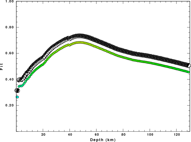
The best fit as a function of depth is given in the following figure:
|
|
Figure 2. Depth sensitivity for waveform mechanism
|
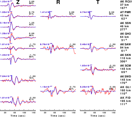
The comparison of the observed and predicted waveforms is given in the next figure. The red traces are the observed and the blue are the predicted.
Each observed-predicted component is plotted to the same scale and peak amplitudes are indicated by the numbers to the left of each trace. A pair of numbers is given in black at the right of each predicted traces. The upper number it the time shift required for maximum correlation between the observed and predicted traces. This time shift is required because the synthetics are not computed at exactly the same distance as the observed, the velocity model used in the predictions may not be perfect and the epicentral parameters may be be off.
A positive time shift indicates that the prediction is too fast and should be delayed to match the observed trace (shift to the right in this figure). A negative value indicates that the prediction is too slow. The lower number gives the percentage of variance reduction to characterize the individual goodness of fit (100% indicates a perfect fit).
The bandpass filter used in the processing and for the display was
cut a -30 a 120
rtr
taper w 0.1
hp c 0.02 n 3
lp c 0.06 n 3
|
|
Figure 3. Waveform comparison for selected depth. Red: observed; Blue - predicted. The time shift with respect to the model prediction is indicated. The percent of fit is also indicated. The time scale is relative to the first trace sample.
|
|
|
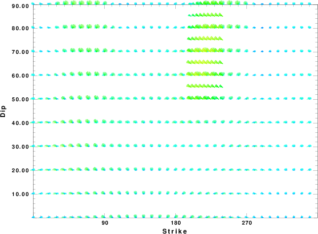
Focal mechanism sensitivity at the preferred depth. The red color indicates a very good fit to the waveforms.
Each solution is plotted as a vector at a given value of strike and dip with the angle of the vector representing the rake angle, measured, with respect to the upward vertical (N) in the figure.
|
A check on the assumed source location is possible by looking at the time shifts between the observed and predicted traces. The time shifts for waveform matching arise for several reasons:
- The origin time and epicentral distance are incorrect
- The velocity model used for the inversion is incorrect
- The velocity model used to define the P-arrival time is not the
same as the velocity model used for the waveform inversion
(assuming that the initial trace alignment is based on the
P arrival time)
Assuming only a mislocation, the time shifts are fit to a functional form:
Time_shift = A + B cos Azimuth + C Sin Azimuth
The time shifts for this inversion lead to the next figure:
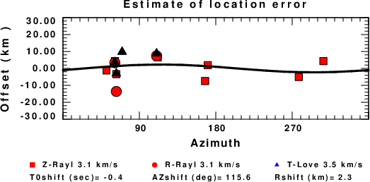
The derived shift in origin time and epicentral coordinates are given at the bottom of the figure.
Velocity Model
The WUS.model used for the waveform synthetic seismograms and for the surface wave eigenfunctions and dispersion is as follows
(The format is in the model96 format of Computer Programs in Seismology).
MODEL.01
Model after     8 iterations
ISOTROPIC
KGS
FLAT EARTH
1-D
CONSTANT VELOCITY
LINE08
LINE09
LINE10
LINE11
      H(KM)   VP(KM/S)   VS(KM/S) RHO(GM/CC)         QP         QS       ETAP       ETAS      FREFP      FREFS
     1.9000     3.4065     2.0089     2.2150  0.302E-02  0.679E-02   0.00       0.00       1.00       1.00
     6.1000     5.5445     3.2953     2.6089  0.349E-02  0.784E-02   0.00       0.00       1.00       1.00
    13.0000     6.2708     3.7396     2.7812  0.212E-02  0.476E-02   0.00       0.00       1.00       1.00
    19.0000     6.4075     3.7680     2.8223  0.111E-02  0.249E-02   0.00       0.00       1.00       1.00
     0.0000     7.9000     4.6200     3.2760  0.164E-10  0.370E-10   0.00       0.00       1.00       1.00
Last Changed Fri Apr 26 07:39:00 PM CDT 2024