Location
Location ANSS
The ANSS event ID is ak0139sm5zgh and the event page is at
https://earthquake.usgs.gov/earthquakes/eventpage/ak0139sm5zgh/executive.
2013/08/01 21:32:47 60.142 -152.916 127.6 4.8 Alaska
Focal Mechanism
 USGS/SLU Moment Tensor Solution
 ENS  2013/08/01 21:32:47:0  60.14 -152.92 127.6 4.8 Alaska

 Stations used:
   AK.BPAW AK.BRLK AK.CAST AK.CNP AK.DHY AK.FID AK.GLI AK.HIN
   AK.KNK AK.KTH AK.PPLA AK.RC01 AK.RND AK.SCM AK.SKN AK.SSN
   AK.SWD AT.OHAK AT.PMR AT.SVW2 II.KDAK

 Filtering commands used:
   cut a -30 a 120
   rtr
   taper w 0.1
   hp c 0.02 n 3
   lp c 0.06 n 3

 Best Fitting Double Couple
  Mo = 2.07e+23 dyne-cm
  Mw = 4.81
  Z  = 130 km
  Plane   Strike  Dip  Rake
   NP1      307    69   148
   NP2       50    60    25
  Principal Axes:
   Axis    Value   Plunge  Azimuth
    T   2.07e+23     38     266
    N   0.00e+00     52      97
    P  -2.07e+23      5       0

 Moment Tensor: (dyne-cm)
    Component   Value
       Mxx    -2.04e+23
       Mxy     9.07e+21
       Mxz    -2.67e+22
       Myy     1.28e+23
       Myz    -9.98e+22
       Mzz     7.56e+22


                     ------ P -----
                 ----------   ---------
              ----------------------------
             ------------------------------
           #####----------------------------#
          ###########-----------------------##
         ################------------------####
        ####################--------------######
        #######################----------#######
       ##########################-------#########
       #######   ##################----##########
       ####### T ####################-###########
       #######   ###################---##########
        ##########################-------#######
        ########################----------######
         #####################-------------####
          #################-----------------##
           ###########----------------------#
             ------------------------------
              ----------------------------
                 ----------------------
                     --------------


 Global CMT Convention Moment Tensor:
      R          T          P
  7.56e+22  -2.67e+22   9.98e+22
 -2.67e+22  -2.04e+23  -9.07e+21
  9.98e+22  -9.07e+21   1.28e+23


Details of the solution is found at

http://www.eas.slu.edu/eqc/eqc_mt/MECH.NA/20130801213247/index.html
|
Preferred Solution
The preferred solution from an analysis of the surface-wave spectral amplitude radiation pattern, waveform inversion or first motion observations is
      STK = 50
      DIP = 60
     RAKE = 25
       MW = 4.81
       HS = 130.0
The NDK file is 20130801213247.ndk
The waveform inversion is preferred.
Magnitudes
Given the availability of digital waveforms for determination of the moment tensor, this section documents the added processing leading to mLg, if appropriate to the region, and ML by application of the respective IASPEI formulae. As a research study, the linear distance term of the IASPEI formula
for ML is adjusted to remove a linear distance trend in residuals to give a regionally defined ML. The defined ML uses horizontal component recordings, but the same procedure is applied to the vertical components since there may be some interest in vertical component ground motions. Residual plots versus distance may indicate interesting features of ground motion scaling in some distance ranges. A residual plot of the regionalized magnitude is given as a function of distance and azimuth, since data sets may transcend different wave propagation provinces.
ML Magnitude
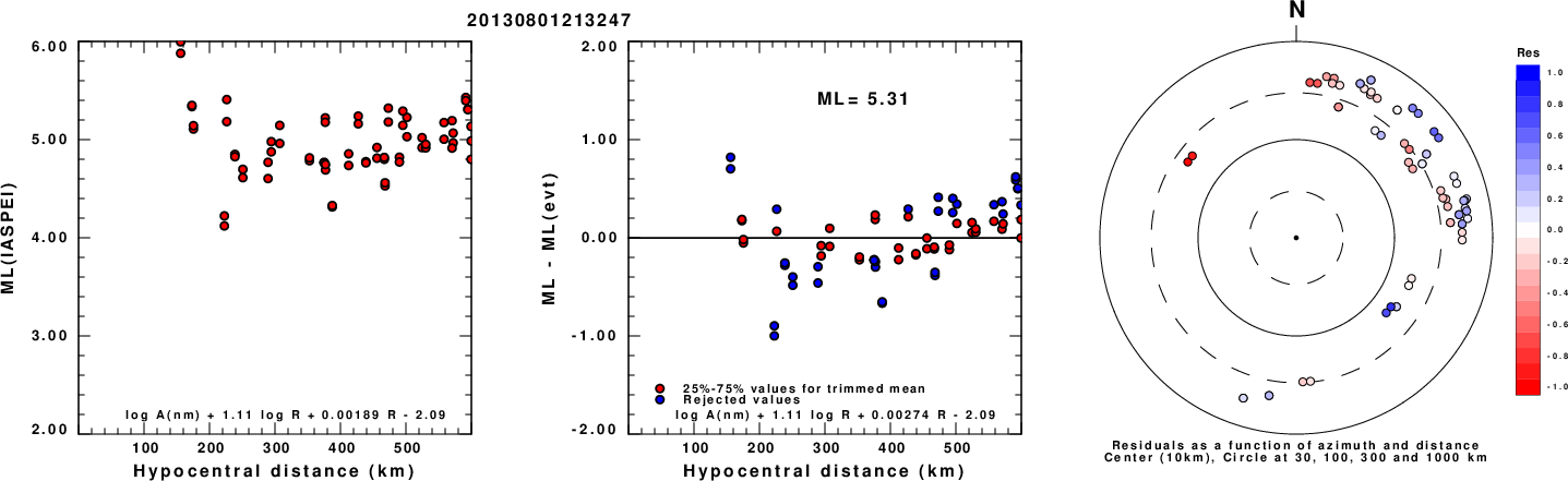
Left: ML computed using the IASPEI formula for Horizontal components. Center: ML residuals computed using a modified IASPEI formula that accounts for path specific attenuation; the values used for the trimmed mean are indicated. The ML relation used for each figure is given at the bottom of each plot.
Right: Residuals from new relation as a function of distance and azimuth.
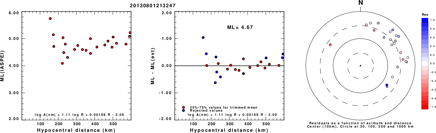
Left: ML computed using the IASPEI formula for Vertical components (research). Center: ML residuals computed using a modified IASPEI formula that accounts for path specific attenuation; the values used for the trimmed mean are indicated. The ML relation used for each figure is given at the bottom of each plot.
Right: Residuals from new relation as a function of distance and azimuth.
Context
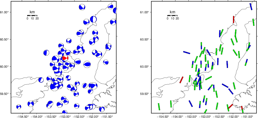
The left panel of the next figure presents the focal mechanism for this earthquake (red) in the context of other nearby events (blue) in the SLU Moment Tensor Catalog. The right panel shows the inferred direction of maximum compressive stress and the type of faulting (green is strike-slip, red is normal, blue is thrust; oblique is shown by a combination of colors). Thus context plot is useful for assessing the appropriateness of the moment tensor of this event.
Waveform Inversion using wvfgrd96
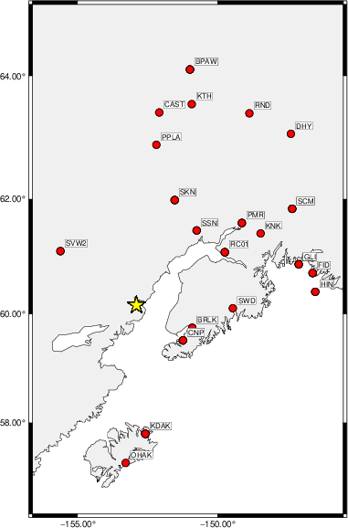
The focal mechanism was determined using broadband seismic waveforms. The location of the event (star) and the
stations used for (red) the waveform inversion are shown in the next figure.
|
|
Location of broadband stations used for waveform inversion
|
The program wvfgrd96 was used with good traces observed at short distance to determine the focal mechanism, depth and seismic moment. This technique requires a high quality signal and well determined velocity model for the Green's functions. To the extent that these are the quality data, this type of mechanism should be preferred over the radiation pattern technique which requires the separate step of defining the pressure and tension quadrants and the correct strike.
The observed and predicted traces are filtered using the following gsac commands:
cut a -30 a 120
rtr
taper w 0.1
hp c 0.02 n 3
lp c 0.06 n 3
The results of this grid search are as follow:
           DEPTH  STK   DIP  RAKE   MW    FIT
WVFGRD96    0.5   115    65   -35   3.86 0.2111
WVFGRD96    1.0   115    65   -35   3.89 0.2239
WVFGRD96    2.0   300    65   -25   3.97 0.2919
WVFGRD96    3.0   305    65   -15   4.00 0.3152
WVFGRD96    4.0   305    75    -5   4.01 0.3344
WVFGRD96    5.0   305    75    -5   4.04 0.3491
WVFGRD96    6.0   305    75     0   4.06 0.3603
WVFGRD96    7.0   305    80    15   4.09 0.3716
WVFGRD96    8.0   310    75    20   4.12 0.3810
WVFGRD96    9.0   310    75    20   4.14 0.3869
WVFGRD96   10.0    40    80    15   4.15 0.3923
WVFGRD96   11.0    40    75    15   4.17 0.4038
WVFGRD96   12.0    40    75    15   4.19 0.4141
WVFGRD96   13.0    40    75    15   4.20 0.4229
WVFGRD96   14.0    40    80    15   4.21 0.4304
WVFGRD96   15.0    40    80    15   4.23 0.4378
WVFGRD96   16.0    40    80    10   4.24 0.4453
WVFGRD96   17.0    40    80    10   4.25 0.4521
WVFGRD96   18.0    40    80    10   4.27 0.4584
WVFGRD96   19.0    40    80    10   4.28 0.4640
WVFGRD96   20.0    40    80    10   4.29 0.4702
WVFGRD96   21.0    40    80    10   4.30 0.4755
WVFGRD96   22.0    40    80    10   4.31 0.4802
WVFGRD96   23.0    40    80    10   4.32 0.4845
WVFGRD96   24.0    40    80    10   4.33 0.4886
WVFGRD96   25.0    40    80    10   4.34 0.4930
WVFGRD96   26.0    40    80    10   4.35 0.4967
WVFGRD96   27.0    40    80    10   4.36 0.4994
WVFGRD96   28.0    40    80    10   4.37 0.5020
WVFGRD96   29.0    40    80    10   4.38 0.5049
WVFGRD96   30.0    40    80    10   4.39 0.5072
WVFGRD96   31.0    40    80    10   4.40 0.5097
WVFGRD96   32.0    40    80    10   4.41 0.5112
WVFGRD96   33.0    40    80    10   4.42 0.5128
WVFGRD96   34.0    40    80    10   4.43 0.5142
WVFGRD96   35.0    40    80    10   4.45 0.5148
WVFGRD96   36.0    40    85     5   4.46 0.5168
WVFGRD96   37.0    40    85     5   4.48 0.5204
WVFGRD96   38.0    40    85     5   4.49 0.5259
WVFGRD96   39.0    40    85     5   4.51 0.5326
WVFGRD96   40.0   220    85   -10   4.54 0.5391
WVFGRD96   41.0    40    85     5   4.55 0.5415
WVFGRD96   42.0    40    90     5   4.56 0.5435
WVFGRD96   43.0    45    85     5   4.57 0.5453
WVFGRD96   44.0   220    90   -10   4.57 0.5469
WVFGRD96   45.0    45    85     5   4.59 0.5493
WVFGRD96   46.0    45    85     5   4.60 0.5512
WVFGRD96   47.0   220    90   -10   4.60 0.5523
WVFGRD96   48.0    40    85    10   4.60 0.5551
WVFGRD96   49.0    40    85    10   4.61 0.5572
WVFGRD96   50.0    40    85    10   4.61 0.5594
WVFGRD96   51.0    45    80     5   4.63 0.5616
WVFGRD96   52.0    45    80     5   4.63 0.5653
WVFGRD96   53.0    45    80     5   4.64 0.5695
WVFGRD96   54.0    45    80     5   4.65 0.5737
WVFGRD96   55.0    45    80     5   4.65 0.5777
WVFGRD96   56.0    45    75     5   4.65 0.5816
WVFGRD96   57.0    45    75     5   4.66 0.5862
WVFGRD96   58.0    45    75     5   4.66 0.5915
WVFGRD96   59.0    45    75     5   4.67 0.5967
WVFGRD96   60.0    45    75     5   4.67 0.6016
WVFGRD96   61.0    45    75    10   4.67 0.6060
WVFGRD96   62.0    45    75    10   4.68 0.6111
WVFGRD96   63.0    45    75    10   4.68 0.6162
WVFGRD96   64.0    45    75    10   4.69 0.6220
WVFGRD96   65.0    45    75    10   4.69 0.6277
WVFGRD96   66.0    45    75    10   4.69 0.6326
WVFGRD96   67.0    45    75    10   4.70 0.6367
WVFGRD96   68.0    45    75    10   4.70 0.6417
WVFGRD96   69.0    45    75    10   4.70 0.6468
WVFGRD96   70.0    45    75    10   4.71 0.6508
WVFGRD96   71.0    50    70    10   4.72 0.6547
WVFGRD96   72.0    50    70    10   4.72 0.6609
WVFGRD96   73.0    50    70    10   4.72 0.6658
WVFGRD96   74.0    50    70    10   4.73 0.6691
WVFGRD96   75.0    50    70    10   4.73 0.6743
WVFGRD96   76.0    50    70    10   4.73 0.6787
WVFGRD96   77.0    50    70    10   4.74 0.6813
WVFGRD96   78.0    50    70    10   4.74 0.6857
WVFGRD96   79.0    50    70    10   4.74 0.6892
WVFGRD96   80.0    50    70    15   4.74 0.6916
WVFGRD96   81.0    50    70    15   4.74 0.6965
WVFGRD96   82.0    50    70    15   4.75 0.6994
WVFGRD96   83.0    50    70    15   4.75 0.7021
WVFGRD96   84.0    50    65    15   4.75 0.7060
WVFGRD96   85.0    50    65    15   4.75 0.7077
WVFGRD96   86.0    50    65    15   4.75 0.7121
WVFGRD96   87.0    50    65    15   4.75 0.7146
WVFGRD96   88.0    50    65    15   4.75 0.7169
WVFGRD96   89.0    50    65    15   4.75 0.7199
WVFGRD96   90.0    50    65    15   4.76 0.7217
WVFGRD96   91.0    50    65    15   4.76 0.7250
WVFGRD96   92.0    50    65    20   4.76 0.7261
WVFGRD96   93.0    50    65    20   4.76 0.7294
WVFGRD96   94.0    50    65    20   4.76 0.7315
WVFGRD96   95.0    50    65    20   4.76 0.7344
WVFGRD96   96.0    50    65    20   4.77 0.7364
WVFGRD96   97.0    50    65    20   4.77 0.7385
WVFGRD96   98.0    50    65    20   4.77 0.7407
WVFGRD96   99.0    50    65    20   4.77 0.7429
WVFGRD96  100.0    50    65    20   4.77 0.7443
WVFGRD96  101.0    50    65    20   4.77 0.7464
WVFGRD96  102.0    50    65    20   4.77 0.7478
WVFGRD96  103.0    50    65    20   4.78 0.7495
WVFGRD96  104.0    50    65    20   4.78 0.7506
WVFGRD96  105.0    50    65    25   4.78 0.7528
WVFGRD96  106.0    50    65    25   4.78 0.7536
WVFGRD96  107.0    50    65    25   4.78 0.7558
WVFGRD96  108.0    50    65    25   4.78 0.7567
WVFGRD96  109.0    50    65    25   4.79 0.7586
WVFGRD96  110.0    50    65    25   4.79 0.7589
WVFGRD96  111.0    50    65    25   4.79 0.7614
WVFGRD96  112.0    50    60    25   4.78 0.7613
WVFGRD96  113.0    50    60    25   4.78 0.7634
WVFGRD96  114.0    50    60    25   4.79 0.7643
WVFGRD96  115.0    50    60    25   4.79 0.7650
WVFGRD96  116.0    50    60    25   4.79 0.7666
WVFGRD96  117.0    50    60    25   4.79 0.7666
WVFGRD96  118.0    50    60    25   4.79 0.7684
WVFGRD96  119.0    50    60    25   4.79 0.7677
WVFGRD96  120.0    50    60    25   4.79 0.7694
WVFGRD96  121.0    50    60    25   4.80 0.7697
WVFGRD96  122.0    50    60    25   4.80 0.7702
WVFGRD96  123.0    50    60    25   4.80 0.7711
WVFGRD96  124.0    50    60    25   4.80 0.7703
WVFGRD96  125.0    50    60    25   4.80 0.7718
WVFGRD96  126.0    50    60    25   4.80 0.7709
WVFGRD96  127.0    50    60    25   4.80 0.7716
WVFGRD96  128.0    50    60    25   4.80 0.7720
WVFGRD96  129.0    50    60    25   4.81 0.7713
WVFGRD96  130.0    50    60    25   4.81 0.7721
WVFGRD96  131.0    50    60    25   4.81 0.7709
WVFGRD96  132.0    50    60    25   4.81 0.7713
WVFGRD96  133.0    50    60    30   4.81 0.7716
WVFGRD96  134.0    50    60    30   4.81 0.7702
WVFGRD96  135.0    50    60    30   4.81 0.7716
WVFGRD96  136.0    50    60    30   4.81 0.7702
WVFGRD96  137.0    50    60    30   4.82 0.7706
WVFGRD96  138.0    50    60    30   4.82 0.7707
WVFGRD96  139.0    50    60    30   4.82 0.7688
The best solution is
WVFGRD96 130.0 50 60 25 4.81 0.7721
The mechanism corresponding to the best fit is
|
|
Figure 1. Waveform inversion focal mechanism
|
The best fit as a function of depth is given in the following figure:
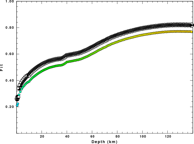
|
|
Figure 2. Depth sensitivity for waveform mechanism
|
The comparison of the observed and predicted waveforms is given in the next figure. The red traces are the observed and the blue are the predicted.
Each observed-predicted component is plotted to the same scale and peak amplitudes are indicated by the numbers to the left of each trace. A pair of numbers is given in black at the right of each predicted traces. The upper number it the time shift required for maximum correlation between the observed and predicted traces. This time shift is required because the synthetics are not computed at exactly the same distance as the observed, the velocity model used in the predictions may not be perfect and the epicentral parameters may be be off.
A positive time shift indicates that the prediction is too fast and should be delayed to match the observed trace (shift to the right in this figure). A negative value indicates that the prediction is too slow. The lower number gives the percentage of variance reduction to characterize the individual goodness of fit (100% indicates a perfect fit).
The bandpass filter used in the processing and for the display was
cut a -30 a 120
rtr
taper w 0.1
hp c 0.02 n 3
lp c 0.06 n 3
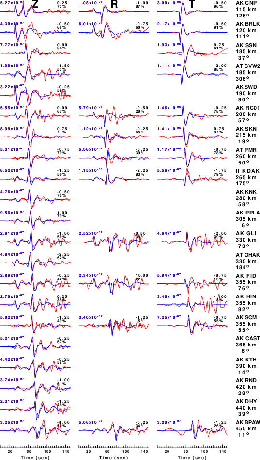
|
|
Figure 3. Waveform comparison for selected depth. Red: observed; Blue - predicted. The time shift with respect to the model prediction is indicated. The percent of fit is also indicated. The time scale is relative to the first trace sample.
|
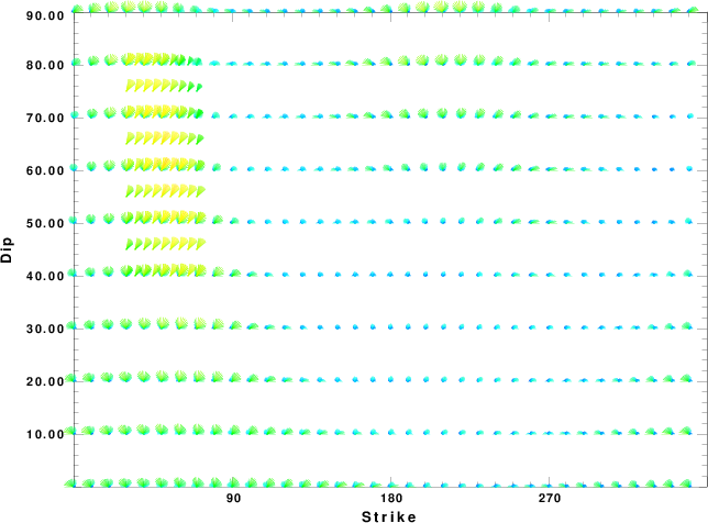
|
|
Focal mechanism sensitivity at the preferred depth. The red color indicates a very good fit to the waveforms.
Each solution is plotted as a vector at a given value of strike and dip with the angle of the vector representing the rake angle, measured, with respect to the upward vertical (N) in the figure.
|
A check on the assumed source location is possible by looking at the time shifts between the observed and predicted traces. The time shifts for waveform matching arise for several reasons:
- The origin time and epicentral distance are incorrect
- The velocity model used for the inversion is incorrect
- The velocity model used to define the P-arrival time is not the
same as the velocity model used for the waveform inversion
(assuming that the initial trace alignment is based on the
P arrival time)
Assuming only a mislocation, the time shifts are fit to a functional form:
Time_shift = A + B cos Azimuth + C Sin Azimuth
The time shifts for this inversion lead to the next figure:
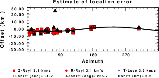
The derived shift in origin time and epicentral coordinates are given at the bottom of the figure.
Velocity Model
The WUS.model used for the waveform synthetic seismograms and for the surface wave eigenfunctions and dispersion is as follows
(The format is in the model96 format of Computer Programs in Seismology).
MODEL.01
Model after     8 iterations
ISOTROPIC
KGS
FLAT EARTH
1-D
CONSTANT VELOCITY
LINE08
LINE09
LINE10
LINE11
      H(KM)   VP(KM/S)   VS(KM/S) RHO(GM/CC)         QP         QS       ETAP       ETAS      FREFP      FREFS
     1.9000     3.4065     2.0089     2.2150  0.302E-02  0.679E-02   0.00       0.00       1.00       1.00
     6.1000     5.5445     3.2953     2.6089  0.349E-02  0.784E-02   0.00       0.00       1.00       1.00
    13.0000     6.2708     3.7396     2.7812  0.212E-02  0.476E-02   0.00       0.00       1.00       1.00
    19.0000     6.4075     3.7680     2.8223  0.111E-02  0.249E-02   0.00       0.00       1.00       1.00
     0.0000     7.9000     4.6200     3.2760  0.164E-10  0.370E-10   0.00       0.00       1.00       1.00
Last Changed Fri Apr 26 07:30:06 PM CDT 2024