Location
Location ANSS
The ANSS event ID is ak01386kg7tb and the event page is at
https://earthquake.usgs.gov/earthquakes/eventpage/ak01386kg7tb/executive.
2013/06/27 11:40:47 61.328 -150.019 55.3 4.2 Alaska
Focal Mechanism
 USGS/SLU Moment Tensor Solution
 ENS  2013/06/27 11:40:47:0  61.33 -150.02  55.3 4.2 Alaska

 Stations used:
   AK.BPAW AK.BWN AK.GHO AK.GLI AK.HDA AK.HIN AK.KNK AK.KTH
   AK.MCK AK.RC01 AK.SAW AK.SCM AK.SKN AK.WRH II.KDAK IU.COLA

 Filtering commands used:
   cut a -10 a 150
   rtr
   taper w 0.1
   hp c 0.02 n 3
   lp c 0.06 n 3

 Best Fitting Double Couple
  Mo = 3.67e+22 dyne-cm
  Mw = 4.31
  Z  = 58 km
  Plane   Strike  Dip  Rake
   NP1      200    65   -35
   NP2      306    59   -150
  Principal Axes:
   Axis    Value   Plunge  Azimuth
    T   3.67e+22      4     254
    N   0.00e+00     48     349
    P  -3.67e+22     42     161

 Moment Tensor: (dyne-cm)
    Component   Value
       Mxx    -1.56e+22
       Mxy     1.57e+22
       Mxz     1.66e+22
       Myy     3.18e+22
       Myz    -8.38e+21
       Mzz    -1.61e+22


                     --------------
                 ---------------#######
              ----------------############
             ---------------###############
           ##########------##################
          ####################################
         ################-----#################
        ################---------###############
        ###############------------#############
       ###############---------------############
       ###############-----------------##########
       ##############-------------------#########
          ###########--------------------########
        T ##########----------------------######
          ##########-----------------------#####
         ###########------------------------###
          #########-----------   -----------##
           ########----------- P ------------
             #######----------   ----------
              ######----------------------
                 ###-------------------
                     --------------


 Global CMT Convention Moment Tensor:
      R          T          P
 -1.61e+22   1.66e+22   8.38e+21
  1.66e+22  -1.56e+22  -1.57e+22
  8.38e+21  -1.57e+22   3.18e+22


Details of the solution is found at

http://www.eas.slu.edu/eqc/eqc_mt/MECH.NA/20130627114047/index.html
|
Preferred Solution
The preferred solution from an analysis of the surface-wave spectral amplitude radiation pattern, waveform inversion or first motion observations is
      STK = 200
      DIP = 65
     RAKE = -35
       MW = 4.31
       HS = 58.0
The NDK file is 20130627114047.ndk
The waveform inversion is preferred.
Moment Tensor Comparison
The following compares this source inversion to those provided by others. The purpose is to look for major differences and also to note slight differences that might be inherent to the processing procedure. For completeness the USGS/SLU solution is repeated from above.
| SLU |
USGSMT |
 USGS/SLU Moment Tensor Solution
 ENS  2013/06/27 11:40:47:0  61.33 -150.02  55.3 4.2 Alaska

 Stations used:
   AK.BPAW AK.BWN AK.GHO AK.GLI AK.HDA AK.HIN AK.KNK AK.KTH
   AK.MCK AK.RC01 AK.SAW AK.SCM AK.SKN AK.WRH II.KDAK IU.COLA

 Filtering commands used:
   cut a -10 a 150
   rtr
   taper w 0.1
   hp c 0.02 n 3
   lp c 0.06 n 3

 Best Fitting Double Couple
  Mo = 3.67e+22 dyne-cm
  Mw = 4.31
  Z  = 58 km
  Plane   Strike  Dip  Rake
   NP1      200    65   -35
   NP2      306    59   -150
  Principal Axes:
   Axis    Value   Plunge  Azimuth
    T   3.67e+22      4     254
    N   0.00e+00     48     349
    P  -3.67e+22     42     161

 Moment Tensor: (dyne-cm)
    Component   Value
       Mxx    -1.56e+22
       Mxy     1.57e+22
       Mxz     1.66e+22
       Myy     3.18e+22
       Myz    -8.38e+21
       Mzz    -1.61e+22


                     --------------
                 ---------------#######
              ----------------############
             ---------------###############
           ##########------##################
          ####################################
         ################-----#################
        ################---------###############
        ###############------------#############
       ###############---------------############
       ###############-----------------##########
       ##############-------------------#########
          ###########--------------------########
        T ##########----------------------######
          ##########-----------------------#####
         ###########------------------------###
          #########-----------   -----------##
           ########----------- P ------------
             #######----------   ----------
              ######----------------------
                 ###-------------------
                     --------------


 Global CMT Convention Moment Tensor:
      R          T          P
 -1.61e+22   1.66e+22   8.38e+21
  1.66e+22  -1.56e+22  -1.57e+22
  8.38e+21  -1.57e+22   3.18e+22


Details of the solution is found at

http://www.eas.slu.edu/eqc/eqc_mt/MECH.NA/20130627114047/index.html
|
us ak10746531-neic-mwr

Type
    Mwr
Moment
    3.62e+15 N-m
Magnitude
    4.3
Percent DC
    77%
Depth
    56.0 km
Author
    neic
Updated
    2013-06-27 16:56:42 UTC

Principal Axes
Axis	Value	Plunge	Azimuth
T	3.413	8	266
N	0.388	40	3
P	-3.801	49	166
Nodal Planes
Plane	Strike	Dip	Rake
NP1	206	64	-45
NP2	320	50	-146
|
|
Magnitudes
Given the availability of digital waveforms for determination of the moment tensor, this section documents the added processing leading to mLg, if appropriate to the region, and ML by application of the respective IASPEI formulae. As a research study, the linear distance term of the IASPEI formula
for ML is adjusted to remove a linear distance trend in residuals to give a regionally defined ML. The defined ML uses horizontal component recordings, but the same procedure is applied to the vertical components since there may be some interest in vertical component ground motions. Residual plots versus distance may indicate interesting features of ground motion scaling in some distance ranges. A residual plot of the regionalized magnitude is given as a function of distance and azimuth, since data sets may transcend different wave propagation provinces.
ML Magnitude
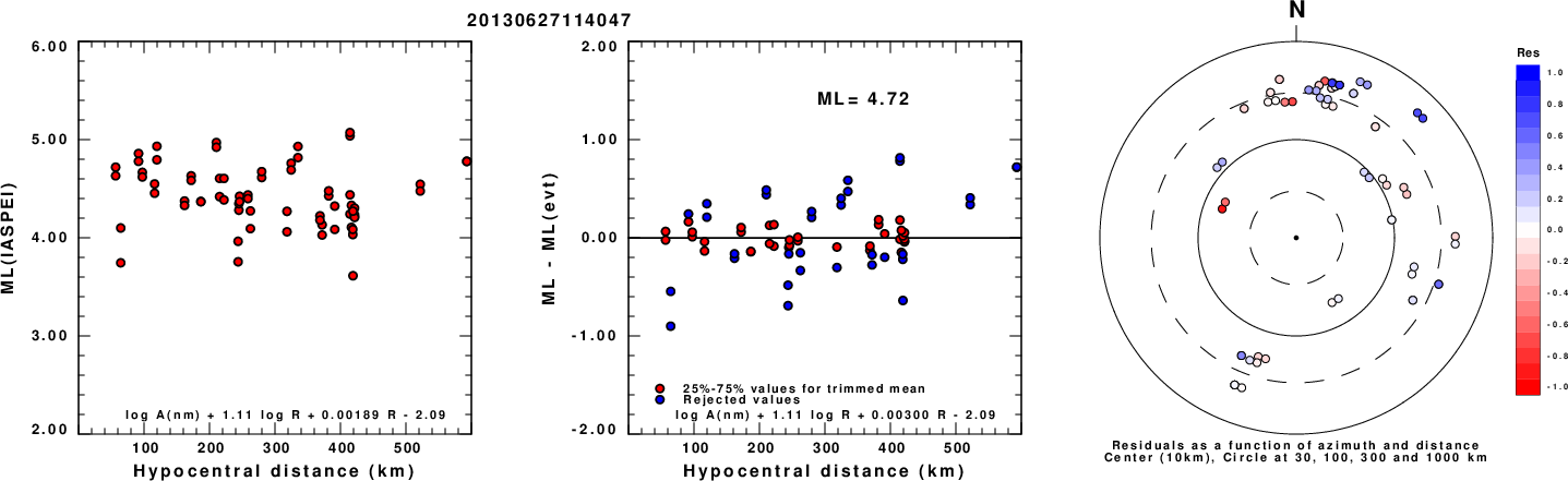
Left: ML computed using the IASPEI formula for Horizontal components. Center: ML residuals computed using a modified IASPEI formula that accounts for path specific attenuation; the values used for the trimmed mean are indicated. The ML relation used for each figure is given at the bottom of each plot.
Right: Residuals from new relation as a function of distance and azimuth.
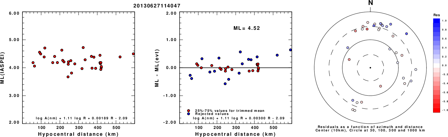
Left: ML computed using the IASPEI formula for Vertical components (research). Center: ML residuals computed using a modified IASPEI formula that accounts for path specific attenuation; the values used for the trimmed mean are indicated. The ML relation used for each figure is given at the bottom of each plot.
Right: Residuals from new relation as a function of distance and azimuth.
Context
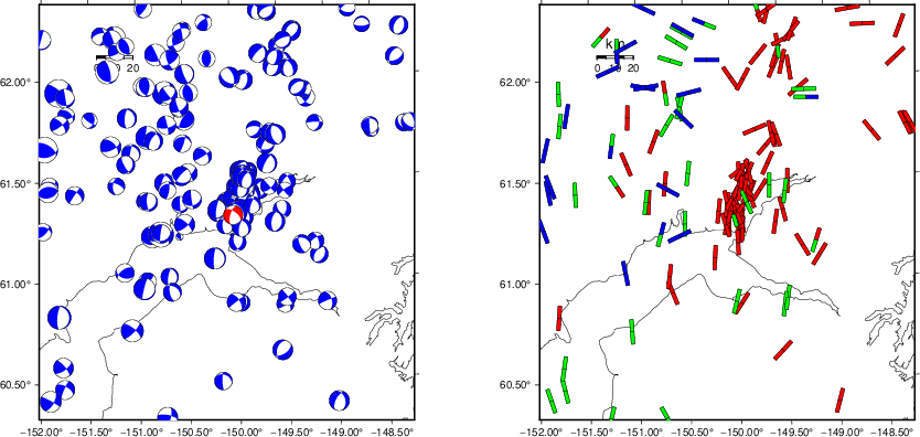
The left panel of the next figure presents the focal mechanism for this earthquake (red) in the context of other nearby events (blue) in the SLU Moment Tensor Catalog. The right panel shows the inferred direction of maximum compressive stress and the type of faulting (green is strike-slip, red is normal, blue is thrust; oblique is shown by a combination of colors). Thus context plot is useful for assessing the appropriateness of the moment tensor of this event.
Waveform Inversion using wvfgrd96
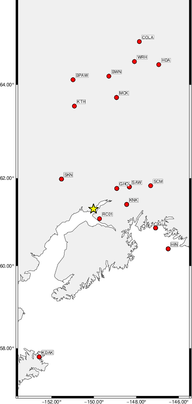
The focal mechanism was determined using broadband seismic waveforms. The location of the event (star) and the
stations used for (red) the waveform inversion are shown in the next figure.
|
|
Location of broadband stations used for waveform inversion
|
The program wvfgrd96 was used with good traces observed at short distance to determine the focal mechanism, depth and seismic moment. This technique requires a high quality signal and well determined velocity model for the Green's functions. To the extent that these are the quality data, this type of mechanism should be preferred over the radiation pattern technique which requires the separate step of defining the pressure and tension quadrants and the correct strike.
The observed and predicted traces are filtered using the following gsac commands:
cut a -10 a 150
rtr
taper w 0.1
hp c 0.02 n 3
lp c 0.06 n 3
The results of this grid search are as follow:
           DEPTH  STK   DIP  RAKE   MW    FIT
WVFGRD96    0.5   160    45    60   3.48 0.1538
WVFGRD96    1.0   160    50    65   3.53 0.1632
WVFGRD96    2.0   165    45    65   3.64 0.2076
WVFGRD96    3.0   160    50    60   3.71 0.2215
WVFGRD96    4.0   160    50    55   3.74 0.2160
WVFGRD96    5.0   150    65    40   3.73 0.2042
WVFGRD96    6.0   305    70   -25   3.72 0.2057
WVFGRD96    7.0   325    85    30   3.74 0.2123
WVFGRD96    8.0   330    80    40   3.79 0.2195
WVFGRD96    9.0   325    85    35   3.80 0.2250
WVFGRD96   10.0   140    90   -35   3.80 0.2289
WVFGRD96   11.0   140    90   -35   3.81 0.2326
WVFGRD96   12.0   320    90    35   3.82 0.2362
WVFGRD96   13.0   305    90    35   3.84 0.2390
WVFGRD96   14.0   305    90    35   3.85 0.2417
WVFGRD96   15.0   305    90    35   3.86 0.2449
WVFGRD96   16.0   305    85    35   3.87 0.2463
WVFGRD96   17.0   305    85    35   3.88 0.2478
WVFGRD96   18.0   305    85    35   3.89 0.2493
WVFGRD96   19.0   305    85    35   3.90 0.2508
WVFGRD96   20.0    40    70   -30   3.90 0.2515
WVFGRD96   21.0    40    70   -30   3.91 0.2579
WVFGRD96   22.0    40    70   -30   3.92 0.2647
WVFGRD96   23.0    40    70   -30   3.93 0.2710
WVFGRD96   24.0    40    70   -30   3.94 0.2768
WVFGRD96   25.0    40    70   -30   3.95 0.2826
WVFGRD96   26.0    40    70   -30   3.96 0.2874
WVFGRD96   27.0    40    70   -30   3.96 0.2923
WVFGRD96   28.0    40    70   -30   3.97 0.2967
WVFGRD96   29.0    40    70   -30   3.98 0.3007
WVFGRD96   30.0    40    70   -25   3.99 0.3048
WVFGRD96   31.0   215    65   -15   4.03 0.3157
WVFGRD96   32.0   215    65   -15   4.04 0.3238
WVFGRD96   33.0   215    65   -20   4.05 0.3317
WVFGRD96   34.0   215    65   -20   4.06 0.3389
WVFGRD96   35.0   215    65   -20   4.07 0.3459
WVFGRD96   36.0   215    65   -20   4.09 0.3523
WVFGRD96   37.0   215    65   -20   4.10 0.3583
WVFGRD96   38.0   215    65   -20   4.11 0.3640
WVFGRD96   39.0   210    65   -20   4.13 0.3704
WVFGRD96   40.0   210    60   -30   4.18 0.3661
WVFGRD96   41.0   210    60   -30   4.19 0.3727
WVFGRD96   42.0   210    60   -30   4.20 0.3783
WVFGRD96   43.0   210    60   -30   4.21 0.3827
WVFGRD96   44.0   210    60   -30   4.22 0.3860
WVFGRD96   45.0   210    60   -30   4.23 0.3891
WVFGRD96   46.0   210    60   -35   4.24 0.3914
WVFGRD96   47.0   210    60   -35   4.24 0.3932
WVFGRD96   48.0   210    60   -35   4.25 0.3943
WVFGRD96   49.0   205    65   -30   4.26 0.3955
WVFGRD96   50.0   205    65   -30   4.27 0.3976
WVFGRD96   51.0   205    65   -30   4.27 0.3991
WVFGRD96   52.0   205    65   -30   4.28 0.4005
WVFGRD96   53.0   205    65   -35   4.28 0.4016
WVFGRD96   54.0   200    65   -35   4.30 0.4024
WVFGRD96   55.0   200    65   -35   4.30 0.4038
WVFGRD96   56.0   200    65   -35   4.30 0.4047
WVFGRD96   57.0   200    65   -35   4.31 0.4054
WVFGRD96   58.0   200    65   -35   4.31 0.4054
WVFGRD96   59.0   200    65   -35   4.32 0.4047
WVFGRD96   60.0   200    65   -35   4.32 0.4037
WVFGRD96   61.0   200    65   -35   4.32 0.4026
WVFGRD96   62.0   200    65   -35   4.32 0.4013
WVFGRD96   63.0   200    65   -35   4.33 0.3992
WVFGRD96   64.0   200    65   -35   4.33 0.3968
WVFGRD96   65.0   200    70   -35   4.34 0.3959
WVFGRD96   66.0   200    70   -35   4.34 0.3953
WVFGRD96   67.0   200    70   -35   4.34 0.3935
WVFGRD96   68.0   200    70   -35   4.35 0.3914
WVFGRD96   69.0   200    70   -35   4.35 0.3899
WVFGRD96   70.0   200    70   -35   4.35 0.3876
WVFGRD96   71.0   200    70   -35   4.35 0.3857
WVFGRD96   72.0   200    70   -35   4.35 0.3831
WVFGRD96   73.0   200    70   -35   4.35 0.3808
WVFGRD96   74.0   200    70   -35   4.35 0.3780
WVFGRD96   75.0   200    70   -35   4.35 0.3754
WVFGRD96   76.0   200    70   -35   4.35 0.3732
WVFGRD96   77.0   200    75   -35   4.37 0.3701
WVFGRD96   78.0   200    75   -35   4.37 0.3684
WVFGRD96   79.0   200    75   -35   4.37 0.3661
The best solution is
WVFGRD96 58.0 200 65 -35 4.31 0.4054
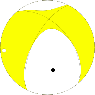
The mechanism corresponding to the best fit is
|
|
Figure 1. Waveform inversion focal mechanism
|
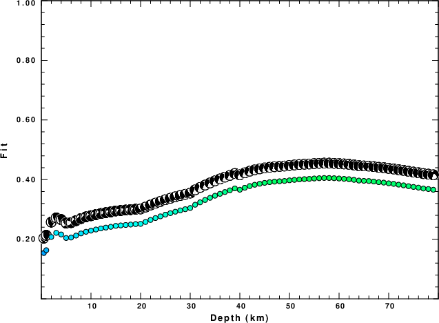
The best fit as a function of depth is given in the following figure:
|
|
Figure 2. Depth sensitivity for waveform mechanism
|
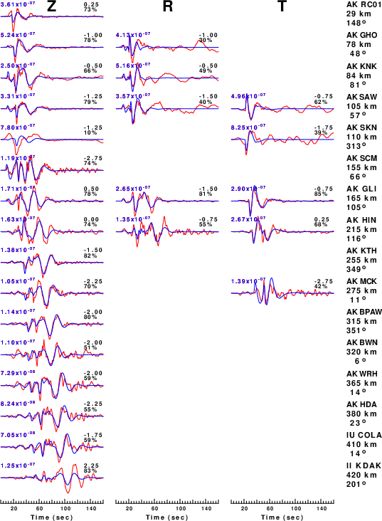
The comparison of the observed and predicted waveforms is given in the next figure. The red traces are the observed and the blue are the predicted.
Each observed-predicted component is plotted to the same scale and peak amplitudes are indicated by the numbers to the left of each trace. A pair of numbers is given in black at the right of each predicted traces. The upper number it the time shift required for maximum correlation between the observed and predicted traces. This time shift is required because the synthetics are not computed at exactly the same distance as the observed, the velocity model used in the predictions may not be perfect and the epicentral parameters may be be off.
A positive time shift indicates that the prediction is too fast and should be delayed to match the observed trace (shift to the right in this figure). A negative value indicates that the prediction is too slow. The lower number gives the percentage of variance reduction to characterize the individual goodness of fit (100% indicates a perfect fit).
The bandpass filter used in the processing and for the display was
cut a -10 a 150
rtr
taper w 0.1
hp c 0.02 n 3
lp c 0.06 n 3
|
|
Figure 3. Waveform comparison for selected depth. Red: observed; Blue - predicted. The time shift with respect to the model prediction is indicated. The percent of fit is also indicated. The time scale is relative to the first trace sample.
|
|
|
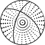
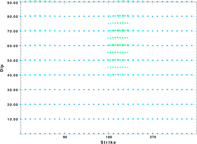
Focal mechanism sensitivity at the preferred depth. The red color indicates a very good fit to the waveforms.
Each solution is plotted as a vector at a given value of strike and dip with the angle of the vector representing the rake angle, measured, with respect to the upward vertical (N) in the figure.
|
A check on the assumed source location is possible by looking at the time shifts between the observed and predicted traces. The time shifts for waveform matching arise for several reasons:
- The origin time and epicentral distance are incorrect
- The velocity model used for the inversion is incorrect
- The velocity model used to define the P-arrival time is not the
same as the velocity model used for the waveform inversion
(assuming that the initial trace alignment is based on the
P arrival time)
Assuming only a mislocation, the time shifts are fit to a functional form:
Time_shift = A + B cos Azimuth + C Sin Azimuth
The time shifts for this inversion lead to the next figure:
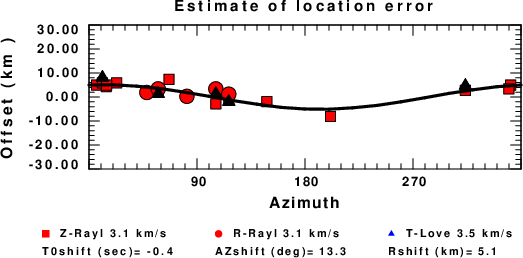
The derived shift in origin time and epicentral coordinates are given at the bottom of the figure.
Velocity Model
The WUS.model used for the waveform synthetic seismograms and for the surface wave eigenfunctions and dispersion is as follows
(The format is in the model96 format of Computer Programs in Seismology).
MODEL.01
Model after     8 iterations
ISOTROPIC
KGS
FLAT EARTH
1-D
CONSTANT VELOCITY
LINE08
LINE09
LINE10
LINE11
      H(KM)   VP(KM/S)   VS(KM/S) RHO(GM/CC)         QP         QS       ETAP       ETAS      FREFP      FREFS
     1.9000     3.4065     2.0089     2.2150  0.302E-02  0.679E-02   0.00       0.00       1.00       1.00
     6.1000     5.5445     3.2953     2.6089  0.349E-02  0.784E-02   0.00       0.00       1.00       1.00
    13.0000     6.2708     3.7396     2.7812  0.212E-02  0.476E-02   0.00       0.00       1.00       1.00
    19.0000     6.4075     3.7680     2.8223  0.111E-02  0.249E-02   0.00       0.00       1.00       1.00
     0.0000     7.9000     4.6200     3.2760  0.164E-10  0.370E-10   0.00       0.00       1.00       1.00
Last Changed Fri Apr 26 06:19:52 PM CDT 2024