The ANSS event ID is usb000h79t and the event page is at https://earthquake.usgs.gov/earthquakes/eventpage/usb000h79t/executive.
2013/05/28 04:36:00 56.198 -120.571 5.0 4.2 British Columbia
USGS/SLU Moment Tensor Solution
ENS 2013/05/28 04:36:00:0 56.20 -120.57 5.0 4.2 British Columbia
Stations used:
AK.JIS CN.BBB CN.BCBC CN.DLBC CN.EDZN CN.FNBB CN.LLLB
CN.MOBC CN.PGC CN.PHC CN.PNT CN.SHB CN.SLEB CN.UBRB CN.WHY
CN.WSLR CN.YKW3 US.WRAK
Filtering commands used:
hp c 0.02 n 3
lp c 0.05 n 3
br c 0.12 0.25 n 4 p 2
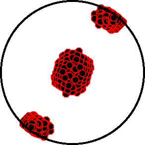
Best Fitting Double Couple
Mo = 1.22e+22 dyne-cm
Mw = 3.99
Z = 2 km
Plane Strike Dip Rake
NP1 314 46 100
NP2 120 45 80
Principal Axes:
Axis Value Plunge Azimuth
T 1.22e+22 83 304
N 0.00e+00 7 127
P -1.22e+22 0 37
Moment Tensor: (dyne-cm)
Component Value
Mxx -7.69e+21
Mxy -5.93e+21
Mxz 7.47e+20
Myy -4.29e+21
Myz -1.29e+21
Mzz 1.20e+22
--------------
----------------------
-------------------------- P
#############--------------
###################---------------
#######################-------------
-#########################------------
--###########################-----------
---############################---------
----############## ############---------
-----############# T #############--------
------############ ##############-------
-------#############################------
--------###########################-----
----------#########################-----
-----------########################---
-------------#####################--
----------------##################
------------------------------
----------------------------
----------------------
--------------
Global CMT Convention Moment Tensor:
R T P
1.20e+22 7.47e+20 1.29e+21
7.47e+20 -7.69e+21 5.93e+21
1.29e+21 5.93e+21 -4.29e+21
Details of the solution is found at
http://www.eas.slu.edu/eqc/eqc_mt/MECH.NA/20130528043600/index.html
|
      STK = 120
      DIP = 45
     RAKE = 80
       MW = 3.99
       HS = 2.0
The NDK file is 20130528043600.ndk The waveform inversion is preferred.
|
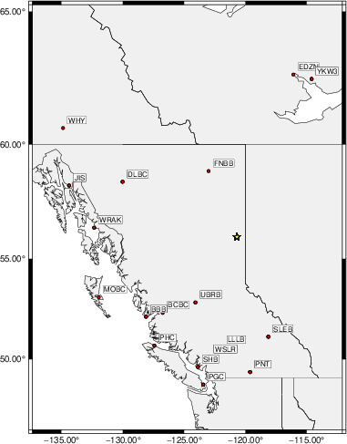
The focal mechanism was determined using broadband seismic waveforms. The location of the event (star) and the stations used for (red) the waveform inversion are shown in the next figure.
|
|
|
The program wvfgrd96 was used with good traces observed at short distance to determine the focal mechanism, depth and seismic moment. This technique requires a high quality signal and well determined velocity model for the Green's functions. To the extent that these are the quality data, this type of mechanism should be preferred over the radiation pattern technique which requires the separate step of defining the pressure and tension quadrants and the correct strike.
The observed and predicted traces are filtered using the following gsac commands:
hp c 0.02 n 3
lp c 0.05 n 3
br c 0.12 0.25 n 4 p 2
The results of this grid search are as follow:
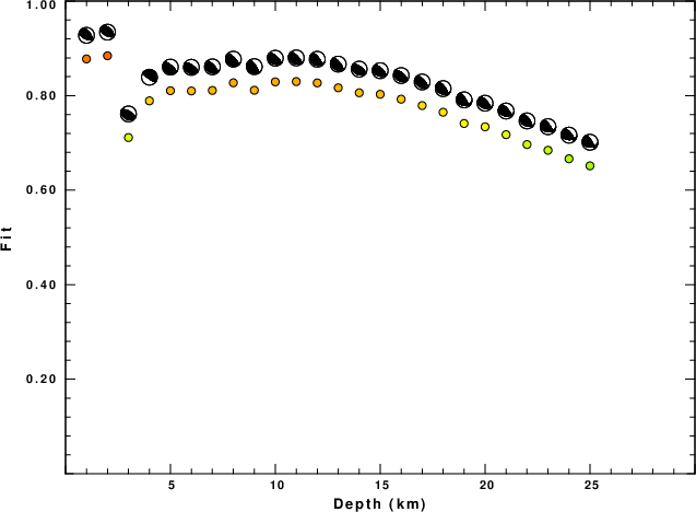
           DEPTH  STK   DIP  RAKE   MW    FIT
WVFGRD96    0.5   115    45    70   3.92 0.6238
WVFGRD96    1.0   315    45   100   3.95 0.6252
WVFGRD96    2.0   120    45    80   3.99 0.6337
WVFGRD96    3.0   305    35    90   4.07 0.6191
WVFGRD96    4.0   120    70    85   4.18 0.5913
WVFGRD96    5.0   120    70    85   4.18 0.5874
WVFGRD96    6.0   120    70    85   4.16 0.5794
WVFGRD96    7.0   120    65    85   4.16 0.5678
WVFGRD96    8.0   120    70    85   4.19 0.5748
WVFGRD96    9.0   310    20    95   4.18 0.5649
WVFGRD96   10.0   105    15    60   4.15 0.5553
WVFGRD96   11.0    95    15    50   4.13 0.5511
WVFGRD96   12.0    55    20     5   4.12 0.5500
WVFGRD96   13.0    40    20   -10   4.11 0.5522
WVFGRD96   14.0    30    20   -20   4.11 0.5551
WVFGRD96   15.0    15    20   -40   4.12 0.5593
WVFGRD96   16.0   140    65   -85   4.14 0.5659
WVFGRD96   17.0   140    60   -80   4.16 0.5770
WVFGRD96   18.0   140    60   -80   4.15 0.5863
WVFGRD96   19.0   140    60   -80   4.15 0.5933
WVFGRD96   20.0   140    60   -75   4.16 0.5969
WVFGRD96   21.0   140    60   -75   4.16 0.5979
WVFGRD96   22.0   140    60   -75   4.16 0.5996
WVFGRD96   23.0   140    55   -75   4.17 0.5997
WVFGRD96   24.0   140    55   -75   4.17 0.5986
WVFGRD96   25.0   140    55   -75   4.17 0.5961
WVFGRD96   26.0   140    55   -75   4.17 0.5931
WVFGRD96   27.0   145    55   -70   4.17 0.5891
WVFGRD96   28.0   145    55   -65   4.18 0.5855
WVFGRD96   29.0   145    55   -65   4.18 0.5814
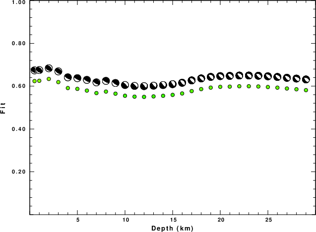
The best solution is
WVFGRD96 2.0 120 45 80 3.99 0.6337
The mechanism corresponding to the best fit is
|
|
|
The best fit as a function of depth is given in the following figure:
|
|
|
The comparison of the observed and predicted waveforms is given in the next figure. The red traces are the observed and the blue are the predicted. Each observed-predicted component is plotted to the same scale and peak amplitudes are indicated by the numbers to the left of each trace. A pair of numbers is given in black at the right of each predicted traces. The upper number it the time shift required for maximum correlation between the observed and predicted traces. This time shift is required because the synthetics are not computed at exactly the same distance as the observed, the velocity model used in the predictions may not be perfect and the epicentral parameters may be be off. A positive time shift indicates that the prediction is too fast and should be delayed to match the observed trace (shift to the right in this figure). A negative value indicates that the prediction is too slow. The lower number gives the percentage of variance reduction to characterize the individual goodness of fit (100% indicates a perfect fit).
The bandpass filter used in the processing and for the display was
hp c 0.02 n 3
lp c 0.05 n 3
br c 0.12 0.25 n 4 p 2
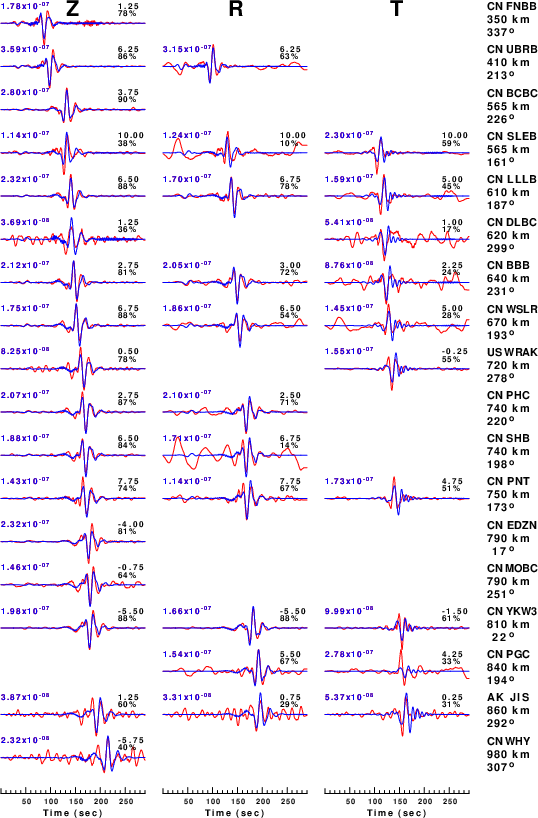
|
| Figure 3. Waveform comparison for selected depth. Red: observed; Blue - predicted. The time shift with respect to the model prediction is indicated. The percent of fit is also indicated. The time scale is relative to the first trace sample. |
|
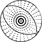
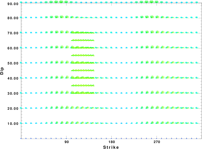
| Focal mechanism sensitivity at the preferred depth. The red color indicates a very good fit to the waveforms. Each solution is plotted as a vector at a given value of strike and dip with the angle of the vector representing the rake angle, measured, with respect to the upward vertical (N) in the figure. |
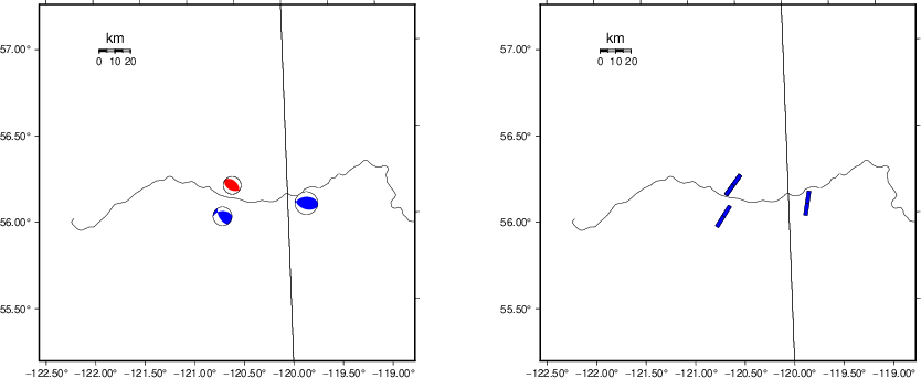
A check on the assumed source location is possible by looking at the time shifts between the observed and predicted traces. The time shifts for waveform matching arise for several reasons:
Time_shift = A + B cos Azimuth + C Sin Azimuth
The time shifts for this inversion lead to the next figure:
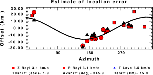
The derived shift in origin time and epicentral coordinates are given at the bottom of the figure.
The following figure shows the stations used in the grid search for the best focal mechanism to fit the surface-wave spectral amplitudes of the Love and Rayleigh waves.

|
|
|
The surface-wave determined focal mechanism is shown here.
  NODAL PLANES


  STK=     119.99
  DIP=      50.00
 RAKE=      80.00

             OR

  STK=     315.33
  DIP=      41.03
 RAKE=     101.70


DEPTH = 2.0 km

Mw = 4.09
Best Fit 0.8844 - P-T axis plot gives solutions with FIT greater than FIT90
 |
Surface wave analysis was performed using codes from Computer Programs in Seismology, specifically the multiple filter analysis program do_mft and the surface-wave radiation pattern search program srfgrd96.
Digital data were collected, instrument response removed and traces converted
to Z, R an T components. Multiple filter analysis was applied to the Z and T traces to obtain the Rayleigh- and Love-wave spectral amplitudes, respectively.
These were input to the search program which examined all depths between 1 and 25 km
and all possible mechanisms.
|
|
|
|
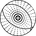
| Pressure-tension axis trends. Since the surface-wave spectra search does not distinguish between P and T axes and since there is a 180 ambiguity in strike, all possible P and T axes are plotted. First motion data and waveforms will be used to select the preferred mechanism. The purpose of this plot is to provide an idea of the possible range of solutions. The P and T-axes for all mechanisms with goodness of fit greater than 0.9 FITMAX (above) are plotted here. |
|
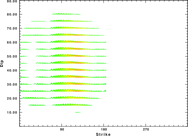
| Focal mechanism sensitivity at the preferred depth. The red color indicates a very good fit to the Love and Rayleigh wave radiation patterns. Each solution is plotted as a vector at a given value of strike and dip with the angle of the vector representing the rake angle, measured, with respect to the upward vertical (N) in the figure. Because of the symmetry of the spectral amplitude rediation patterns, only strikes from 0-180 degrees are sampled. |
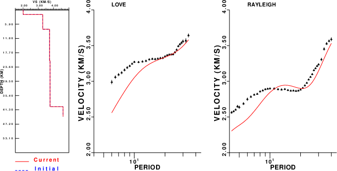
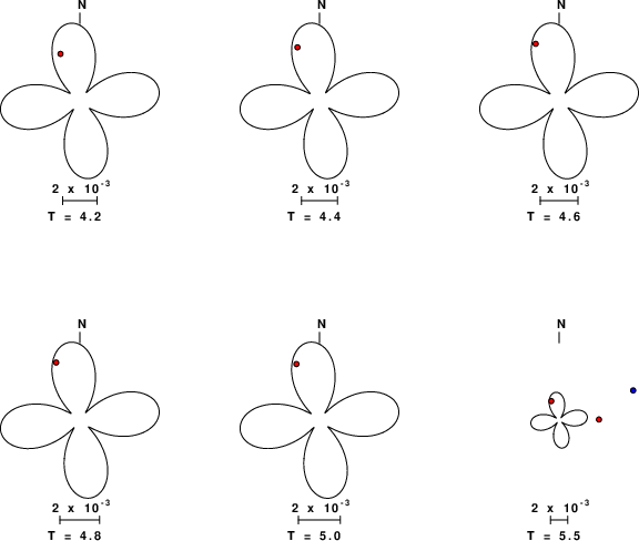
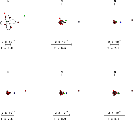
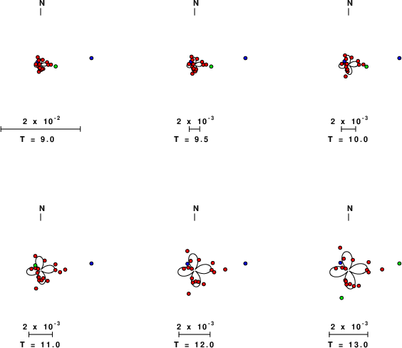
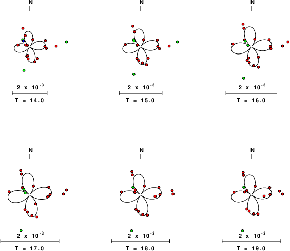
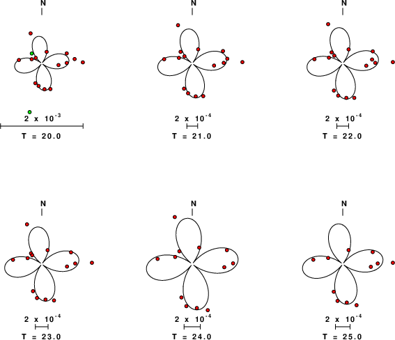
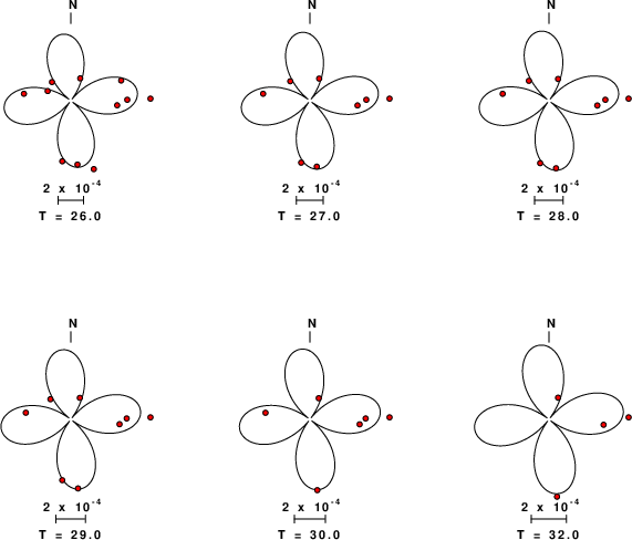
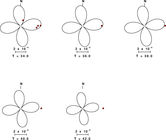
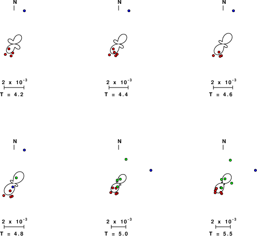
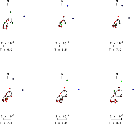
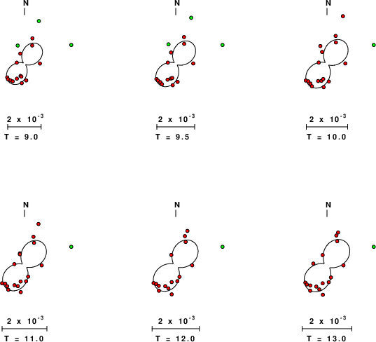
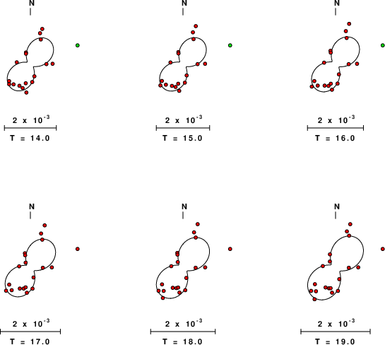
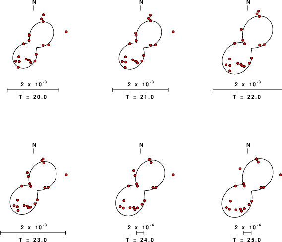
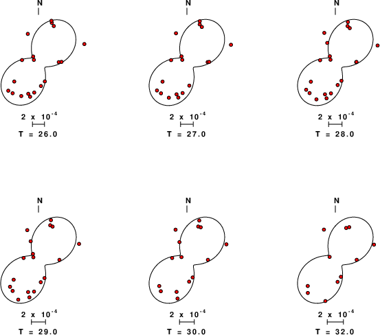
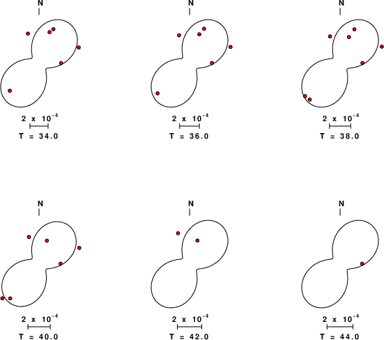
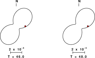
The next set of figures compares the observed and predicted surface wave radiation patterns as a function of period. The observed spectral amplitude have been corrected for anleastic attenuation by multiplication by a factor of eγr and corrected for surface wave geometrical spreading to a reference distance of 1000km. If the theoretical γ values are not perfect, then observations at large distance will plot as outliers.
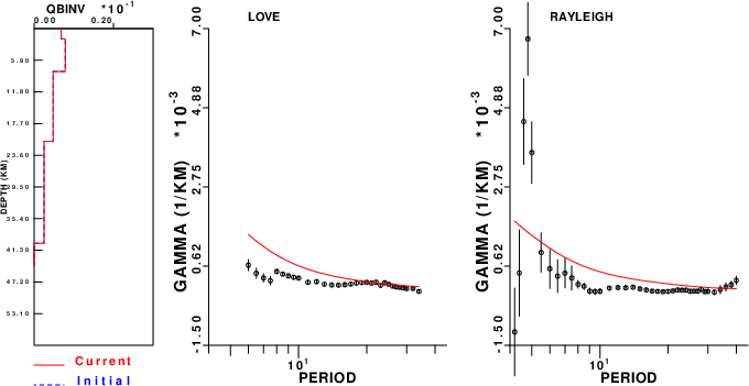
Given the mechanisms and depth, the observed spectral amplitudes can be compared to the theoretical predictions of a model with infinite Q. The difference can be used to estimated the anelastic attenuation coefficent at each period according to the model
Obs = e-γ r PreThe γ values can be use to invert for the Q structure. The next figure compares the network average group velocities to those of the model and as well as the γ derived from this data set and that of the model.
|
|
The WUS.model used for the waveform synthetic seismograms and for the surface wave eigenfunctions and dispersion is as follows (The format is in the model96 format of Computer Programs in Seismology).
MODEL.01
Model after     8 iterations
ISOTROPIC
KGS
FLAT EARTH
1-D
CONSTANT VELOCITY
LINE08
LINE09
LINE10
LINE11
      H(KM)   VP(KM/S)   VS(KM/S) RHO(GM/CC)         QP         QS       ETAP       ETAS      FREFP      FREFS
     1.9000     3.4065     2.0089     2.2150  0.302E-02  0.679E-02   0.00       0.00       1.00       1.00
     6.1000     5.5445     3.2953     2.6089  0.349E-02  0.784E-02   0.00       0.00       1.00       1.00
    13.0000     6.2708     3.7396     2.7812  0.212E-02  0.476E-02   0.00       0.00       1.00       1.00
    19.0000     6.4075     3.7680     2.8223  0.111E-02  0.249E-02   0.00       0.00       1.00       1.00
     0.0000     7.9000     4.6200     3.2760  0.164E-10  0.370E-10   0.00       0.00       1.00       1.00