Location
SLU Location
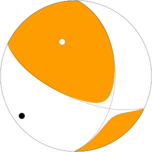
To check the ANSS location or to compare the observed P-wave first motions to the moment tensor solution, P- and S-wave first arrival times were manually read together with the P-wave first motions. The subsequent output of the program elocate is given in the file elocate.txt. The first motion plot is shown below.
Location ANSS
The ANSS event ID is ld60040526 and the event page is at
https://earthquake.usgs.gov/earthquakes/eventpage/ld60040526/executive.
2013/05/17 13:43:23 45.757 -76.353 13.0 5.06 Ontario
Focal Mechanism
 USGS/SLU Moment Tensor Solution
 ENS  2013/05/17 13:43:23:0  45.76  -76.35  13.0 5.1 Ontario

 Stations used:
   CN.A16 CN.A21 CN.A54 CN.A61 CN.A64 CN.ACTO CN.ALFO CN.BANO
   CN.BMRO CN.BRCO CN.BUKO CN.BWLO CN.CHGQ CN.DELO CN.DMCQ
   CN.DRCO CN.GAC CN.KAPO CN.KGNO CN.KILO CN.KLBO CN.LATQ
   CN.LMQ CN.LSQQ CN.MATQ CN.MEDO CN.MNTQ CN.ORIO CN.OTT
   CN.PECO CN.PKRO CN.PLVO CN.SADO CN.STCO CN.SUNO CN.TOBO
   CN.TORO CN.VABQ CN.VLDQ IU.HRV IU.SSPA LD.ACCN LD.ALLY
   LD.BRNJ LD.FRNY LD.KSCT LD.KSPA LD.LUPA LD.NCB LD.ODNJ
   LD.PAL LD.WVNY NE.BCX NE.HNH NE.QUA2 NE.TRY NE.VT1 NE.WES
   NE.WSPT NE.WVL NE.YLE TA.D47A TA.D48A TA.D49A TA.D51A
   TA.D52A TA.D54A TA.E46A TA.E47A TA.E50A TA.E51A TA.E52A
   TA.E53A TA.E54A TA.F48A TA.F49A TA.F51A TA.F52A TA.G47A
   TA.G53A TA.H48A TA.H52A TA.H55A TA.H56A TA.I47A TA.I49A
   TA.I51A TA.I52A TA.I53A TA.I55A TA.J48A TA.J52A TA.J54A
   TA.J55A TA.K50A TA.K51A TA.K52A TA.K55A TA.L53A TA.L55A
   TA.M52A TA.M53A TA.M54A TA.M55A TA.M65A TA.N53A TA.N54A
   TA.N55A TA.N59A TA.O56A TA.P60A US.BINY US.ERPA US.GLMI
   US.LBNH US.LONY US.PKME

 Filtering commands used:
   hp c 0.02 n 3
   lp c 0.10 n 3

 Best Fitting Double Couple
  Mo = 6.84e+22 dyne-cm
  Mw = 4.49
  Z  = 13 km
  Plane   Strike  Dip  Rake
   NP1      135    50    65
   NP2      351    46   117
  Principal Axes:
   Axis    Value   Plunge  Azimuth
    T   6.84e+22     71     338
    N   0.00e+00     19     152
    P  -6.84e+22      2     242

 Moment Tensor: (dyne-cm)
    Component   Value
       Mxx    -8.38e+21
       Mxy    -3.05e+22
       Mxz     2.07e+22
       Myy    -5.27e+22
       Myz    -5.53e+21
       Mzz     6.10e+22


                     ######--------
                 #############---------
              ##################----------
             #####################---------
           --######################----------
          ---#######################----------
         ----########################----------
        -----############   ##########----------
        ------########### T ##########----------
       -------###########   ###########----------
       --------########################----------
       ---------#######################----------
       ----------######################----------
        -----------####################---------
        ------------###################---------
            ----------#################--------
          P ------------##############--------
            ---------------###########-------
             ------------------######------
              ----------------------######
                 -----------------#####
                     ------------##


 Global CMT Convention Moment Tensor:
      R          T          P
  6.10e+22   2.07e+22   5.53e+21
  2.07e+22  -8.38e+21   3.05e+22
  5.53e+21   3.05e+22  -5.27e+22


Details of the solution is found at

http://www.eas.slu.edu/eqc/eqc_mt/MECH.NA/20130517134323/index.html
|
Preferred Solution
The preferred solution from an analysis of the surface-wave spectral amplitude radiation pattern, waveform inversion or first motion observations is
      STK = 135
      DIP = 50
     RAKE = 65
       MW = 4.49
       HS = 13.0
The NDK file is 20130517134323.ndk
The waveform inversion is preferred.
Moment Tensor Comparison
The following compares this source inversion to those provided by others. The purpose is to look for major differences and also to note slight differences that might be inherent to the processing procedure. For completeness the USGS/SLU solution is repeated from above.
| SLU |
USGSMT |
 USGS/SLU Moment Tensor Solution
 ENS  2013/05/17 13:43:23:0  45.76  -76.35  13.0 5.1 Ontario

 Stations used:
   CN.A16 CN.A21 CN.A54 CN.A61 CN.A64 CN.ACTO CN.ALFO CN.BANO
   CN.BMRO CN.BRCO CN.BUKO CN.BWLO CN.CHGQ CN.DELO CN.DMCQ
   CN.DRCO CN.GAC CN.KAPO CN.KGNO CN.KILO CN.KLBO CN.LATQ
   CN.LMQ CN.LSQQ CN.MATQ CN.MEDO CN.MNTQ CN.ORIO CN.OTT
   CN.PECO CN.PKRO CN.PLVO CN.SADO CN.STCO CN.SUNO CN.TOBO
   CN.TORO CN.VABQ CN.VLDQ IU.HRV IU.SSPA LD.ACCN LD.ALLY
   LD.BRNJ LD.FRNY LD.KSCT LD.KSPA LD.LUPA LD.NCB LD.ODNJ
   LD.PAL LD.WVNY NE.BCX NE.HNH NE.QUA2 NE.TRY NE.VT1 NE.WES
   NE.WSPT NE.WVL NE.YLE TA.D47A TA.D48A TA.D49A TA.D51A
   TA.D52A TA.D54A TA.E46A TA.E47A TA.E50A TA.E51A TA.E52A
   TA.E53A TA.E54A TA.F48A TA.F49A TA.F51A TA.F52A TA.G47A
   TA.G53A TA.H48A TA.H52A TA.H55A TA.H56A TA.I47A TA.I49A
   TA.I51A TA.I52A TA.I53A TA.I55A TA.J48A TA.J52A TA.J54A
   TA.J55A TA.K50A TA.K51A TA.K52A TA.K55A TA.L53A TA.L55A
   TA.M52A TA.M53A TA.M54A TA.M55A TA.M65A TA.N53A TA.N54A
   TA.N55A TA.N59A TA.O56A TA.P60A US.BINY US.ERPA US.GLMI
   US.LBNH US.LONY US.PKME

 Filtering commands used:
   hp c 0.02 n 3
   lp c 0.10 n 3

 Best Fitting Double Couple
  Mo = 6.84e+22 dyne-cm
  Mw = 4.49
  Z  = 13 km
  Plane   Strike  Dip  Rake
   NP1      135    50    65
   NP2      351    46   117
  Principal Axes:
   Axis    Value   Plunge  Azimuth
    T   6.84e+22     71     338
    N   0.00e+00     19     152
    P  -6.84e+22      2     242

 Moment Tensor: (dyne-cm)
    Component   Value
       Mxx    -8.38e+21
       Mxy    -3.05e+22
       Mxz     2.07e+22
       Myy    -5.27e+22
       Myz    -5.53e+21
       Mzz     6.10e+22


                     ######--------
                 #############---------
              ##################----------
             #####################---------
           --######################----------
          ---#######################----------
         ----########################----------
        -----############   ##########----------
        ------########### T ##########----------
       -------###########   ###########----------
       --------########################----------
       ---------#######################----------
       ----------######################----------
        -----------####################---------
        ------------###################---------
            ----------#################--------
          P ------------##############--------
            ---------------###########-------
             ------------------######------
              ----------------------######
                 -----------------#####
                     ------------##


 Global CMT Convention Moment Tensor:
      R          T          P
  6.10e+22   2.07e+22   5.53e+21
  2.07e+22  -8.38e+21   3.05e+22
  5.53e+21   3.05e+22  -5.27e+22


Details of the solution is found at

http://www.eas.slu.edu/eqc/eqc_mt/MECH.NA/20130517134323/index.html
|
us usb000gxna-neic-mwr

Type
    Mwr
Moment
    4.97e+15 N-m
Magnitude
    4.4
Percent DC
    92%
Depth
    10.0 km
Author
    neic
Updated
    2013-05-17 14:39:09 UTC

Principal Axes
Axis	Value	Plunge	Azimuth
T	5.064	50°	338°
N	-0.188	38°	134°
P	-4.876	12°	234°
Nodal Planes
Plane	Strike	Dip	Rake
NP1	115°	67°	48°
NP2	1°	47°	147°
|
Magnitudes
Given the availability of digital waveforms for determination of the moment tensor, this section documents the added processing leading to mLg, if appropriate to the region, and ML by application of the respective IASPEI formulae. As a research study, the linear distance term of the IASPEI formula
for ML is adjusted to remove a linear distance trend in residuals to give a regionally defined ML. The defined ML uses horizontal component recordings, but the same procedure is applied to the vertical components since there may be some interest in vertical component ground motions. Residual plots versus distance may indicate interesting features of ground motion scaling in some distance ranges. A residual plot of the regionalized magnitude is given as a function of distance and azimuth, since data sets may transcend different wave propagation provinces.
mLg Magnitude
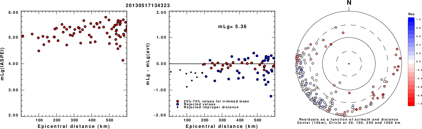
Left: mLg computed using the IASPEI formula. Center: mLg residuals versus epicentral distance ; the values used for the trimmed mean magnitude estimate are indicated.
Right: residuals as a function of distance and azimuth.
ML Magnitude
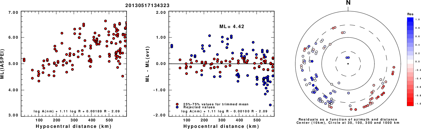
Left: ML computed using the IASPEI formula for Horizontal components. Center: ML residuals computed using a modified IASPEI formula that accounts for path specific attenuation; the values used for the trimmed mean are indicated. The ML relation used for each figure is given at the bottom of each plot.
Right: Residuals from new relation as a function of distance and azimuth.
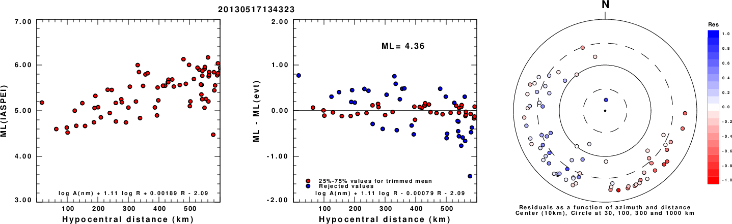
Left: ML computed using the IASPEI formula for Vertical components (research). Center: ML residuals computed using a modified IASPEI formula that accounts for path specific attenuation; the values used for the trimmed mean are indicated. The ML relation used for each figure is given at the bottom of each plot.
Right: Residuals from new relation as a function of distance and azimuth.
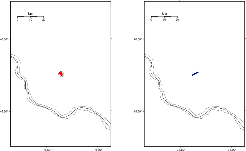
Context
The left panel of the next figure presents the focal mechanism for this earthquake (red) in the context of other nearby events (blue) in the SLU Moment Tensor Catalog. The right panel shows the inferred direction of maximum compressive stress and the type of faulting (green is strike-slip, red is normal, blue is thrust; oblique is shown by a combination of colors). Thus context plot is useful for assessing the appropriateness of the moment tensor of this event.
Waveform Inversion using wvfgrd96
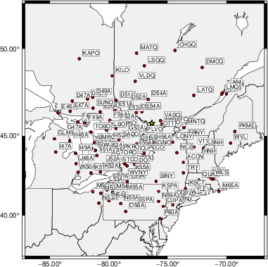
The focal mechanism was determined using broadband seismic waveforms. The location of the event (star) and the
stations used for (red) the waveform inversion are shown in the next figure.
|
|
Location of broadband stations used for waveform inversion
|
The program wvfgrd96 was used with good traces observed at short distance to determine the focal mechanism, depth and seismic moment. This technique requires a high quality signal and well determined velocity model for the Green's functions. To the extent that these are the quality data, this type of mechanism should be preferred over the radiation pattern technique which requires the separate step of defining the pressure and tension quadrants and the correct strike.
The observed and predicted traces are filtered using the following gsac commands:
hp c 0.02 n 3
lp c 0.10 n 3
The results of this grid search are as follow:
           DEPTH  STK   DIP  RAKE   MW    FIT
WVFGRD96    0.5    75    45   -90   4.29 0.5340
WVFGRD96    1.0    75    45   -90   4.34 0.5375
WVFGRD96    2.0    95    70   -65   4.43 0.5071
WVFGRD96    3.0   100    75   -60   4.40 0.5057
WVFGRD96    4.0   100    75   -60   4.39 0.5134
WVFGRD96    5.0   100    75   -55   4.38 0.5279
WVFGRD96    6.0   160    30   100   4.41 0.5584
WVFGRD96    7.0   135    40    65   4.43 0.6096
WVFGRD96    8.0   135    45    65   4.44 0.6537
WVFGRD96    9.0   130    50    60   4.45 0.6868
WVFGRD96   10.0   135    50    65   4.48 0.7040
WVFGRD96   11.0   135    50    65   4.48 0.7236
WVFGRD96   12.0   135    50    65   4.49 0.7333
WVFGRD96   13.0   135    50    65   4.49 0.7353
WVFGRD96   14.0   130    55    60   4.50 0.7322
WVFGRD96   15.0   130    55    60   4.50 0.7253
WVFGRD96   16.0   130    55    60   4.51 0.7151
WVFGRD96   17.0   130    55    60   4.52 0.7019
WVFGRD96   18.0   130    55    60   4.52 0.6868
WVFGRD96   19.0   130    55    60   4.53 0.6697
WVFGRD96   20.0   135    55    65   4.55 0.6501
WVFGRD96   21.0   130    60    60   4.56 0.6320
WVFGRD96   22.0   130    60    65   4.56 0.6132
WVFGRD96   23.0   130    60    65   4.57 0.5934
WVFGRD96   24.0   130    60    65   4.57 0.5729
WVFGRD96   25.0   130    60    65   4.58 0.5517
WVFGRD96   26.0   130    60    65   4.58 0.5296
WVFGRD96   27.0   125    65    60   4.58 0.5073
WVFGRD96   28.0   125    65    60   4.58 0.4884
WVFGRD96   29.0   125    55    50   4.58 0.4740
The best solution is
WVFGRD96 13.0 135 50 65 4.49 0.7353
The mechanism corresponding to the best fit is
|
|
Figure 1. Waveform inversion focal mechanism
|
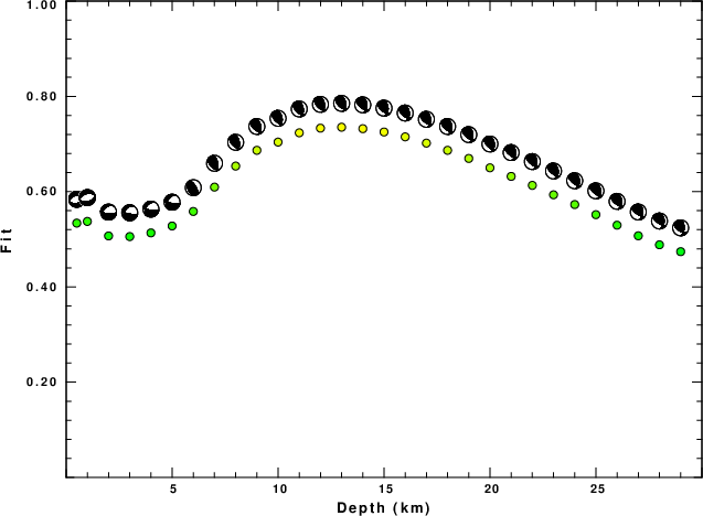
The best fit as a function of depth is given in the following figure:
|
|
Figure 2. Depth sensitivity for waveform mechanism
|
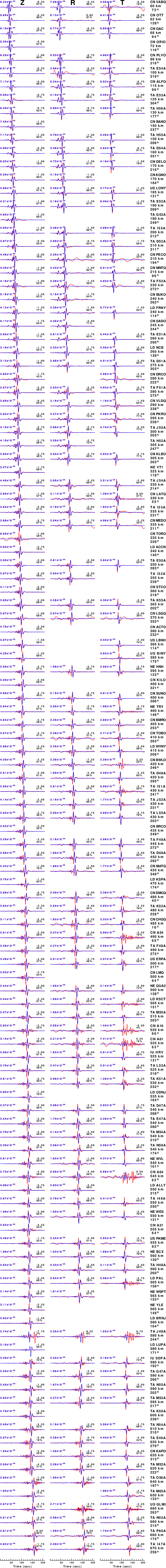
The comparison of the observed and predicted waveforms is given in the next figure. The red traces are the observed and the blue are the predicted.
Each observed-predicted component is plotted to the same scale and peak amplitudes are indicated by the numbers to the left of each trace. A pair of numbers is given in black at the right of each predicted traces. The upper number it the time shift required for maximum correlation between the observed and predicted traces. This time shift is required because the synthetics are not computed at exactly the same distance as the observed, the velocity model used in the predictions may not be perfect and the epicentral parameters may be be off.
A positive time shift indicates that the prediction is too fast and should be delayed to match the observed trace (shift to the right in this figure). A negative value indicates that the prediction is too slow. The lower number gives the percentage of variance reduction to characterize the individual goodness of fit (100% indicates a perfect fit).
The bandpass filter used in the processing and for the display was
hp c 0.02 n 3
lp c 0.10 n 3
|
|
Figure 3. Waveform comparison for selected depth. Red: observed; Blue - predicted. The time shift with respect to the model prediction is indicated. The percent of fit is also indicated. The time scale is relative to the first trace sample.
|
|
|
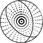
Focal mechanism sensitivity at the preferred depth. The red color indicates a very good fit to the waveforms.
Each solution is plotted as a vector at a given value of strike and dip with the angle of the vector representing the rake angle, measured, with respect to the upward vertical (N) in the figure.
|
A check on the assumed source location is possible by looking at the time shifts between the observed and predicted traces. The time shifts for waveform matching arise for several reasons:
- The origin time and epicentral distance are incorrect
- The velocity model used for the inversion is incorrect
- The velocity model used to define the P-arrival time is not the
same as the velocity model used for the waveform inversion
(assuming that the initial trace alignment is based on the
P arrival time)
Assuming only a mislocation, the time shifts are fit to a functional form:
Time_shift = A + B cos Azimuth + C Sin Azimuth
The time shifts for this inversion lead to the next figure:
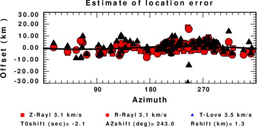
The derived shift in origin time and epicentral coordinates are given at the bottom of the figure.
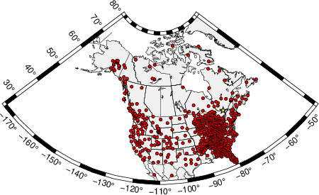
Surface-Wave Focal Mechanism
The following figure shows the stations used in the grid search for the best focal mechanism to fit the surface-wave spectral amplitudes of the Love and Rayleigh waves.
|
|
Location of broadband stations used to obtain focal mechanism from surface-wave spectral amplitudes
|
The surface-wave determined focal mechanism is shown here.
  NODAL PLANES


  STK=     134.99
  DIP=      50.00
 RAKE=      64.99

             OR

  STK=     350.95
  DIP=      46.04
 RAKE=     116.73


DEPTH = 10.0 km

Mw = 4.61
Best Fit 0.8702 - P-T axis plot gives solutions with FIT greater than FIT90
Surface-wave analysis
Surface wave analysis was performed using codes from
Computer Programs in Seismology, specifically the
multiple filter analysis program do_mft and the surface-wave
radiation pattern search program srfgrd96.
Data preparation
Digital data were collected, instrument response removed and traces converted
to Z, R an T components. Multiple filter analysis was applied to the Z and T traces to obtain the Rayleigh- and Love-wave spectral amplitudes, respectively.
These were input to the search program which examined all depths between 1 and 25 km
and all possible mechanisms.
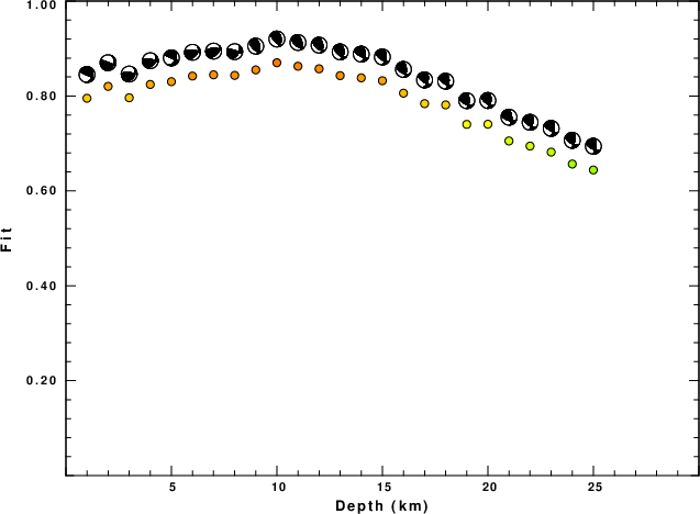
|
|
Best mechanism fit as a function of depth. The preferred depth is given above. Lower hemisphere projection
|

|
|
Pressure-tension axis trends. Since the surface-wave spectra search does not distinguish between P and T axes and since there is a 180 ambiguity in strike, all possible P and T axes are plotted. First motion data and waveforms will be used to select the preferred mechanism. The purpose of this plot is to provide an idea of the
possible range of solutions. The P and T-axes for all mechanisms with goodness of fit greater than 0.9 FITMAX (above) are plotted here.
|
|
|
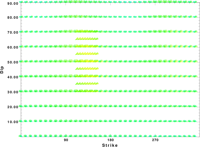
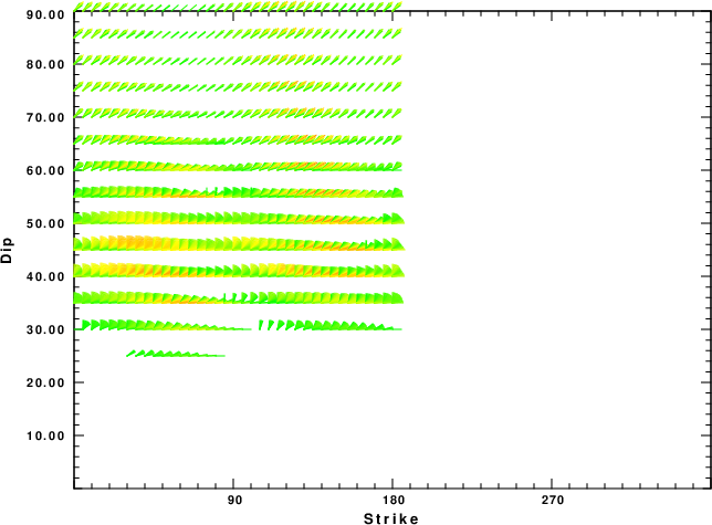
Focal mechanism sensitivity at the preferred depth. The red color indicates a very good fit to the Love and Rayleigh wave radiation patterns.
Each solution is plotted as a vector at a given value of strike and dip with the angle of the vector representing the rake angle, measured, with respect to the upward vertical (N) in the figure. Because of the symmetry of the spectral amplitude rediation patterns, only strikes from 0-180 degrees are sampled.
|
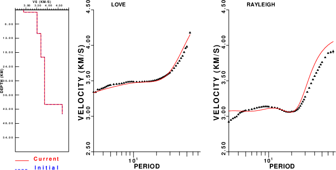
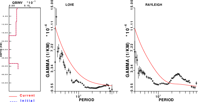
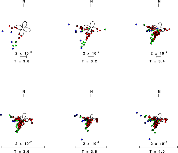
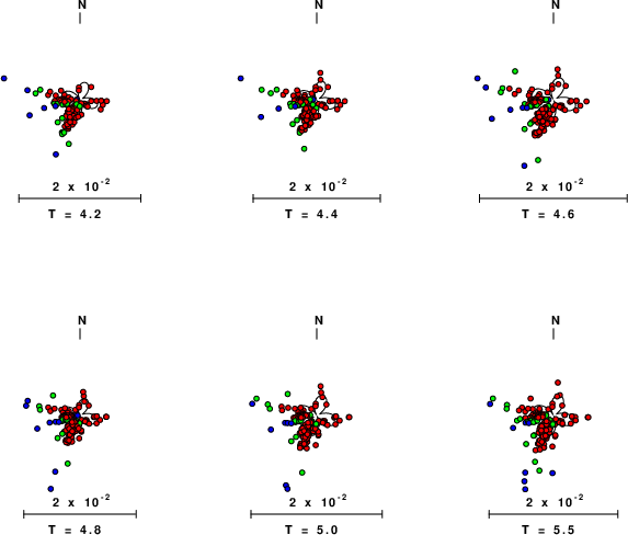
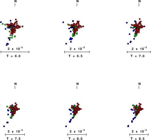
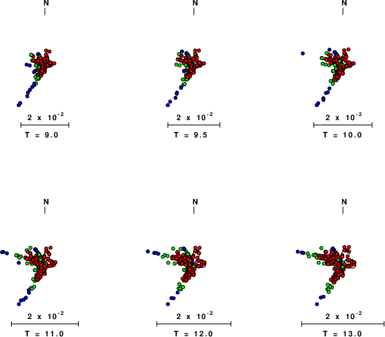
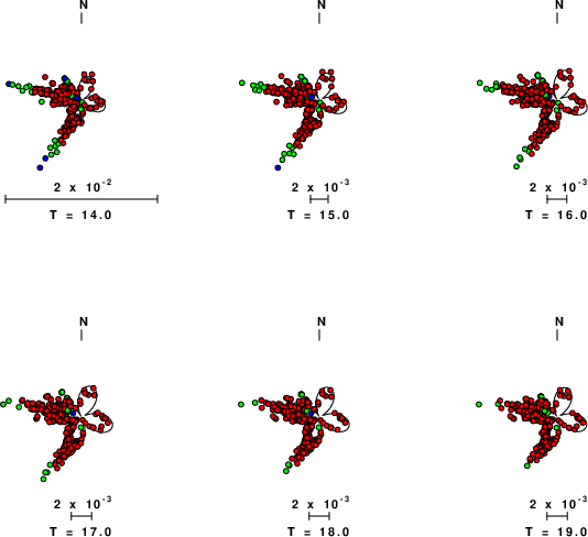
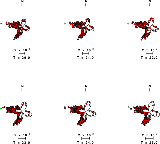
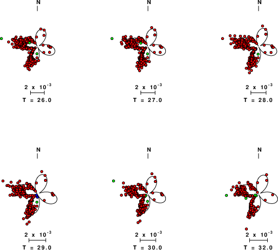
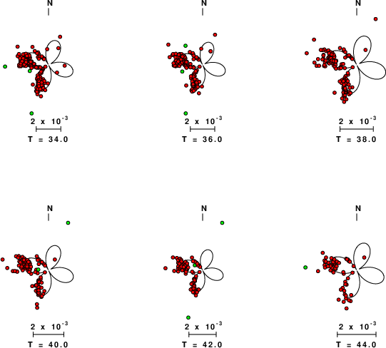
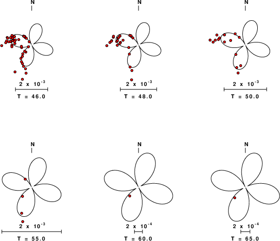
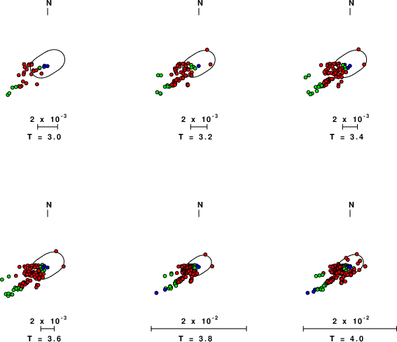
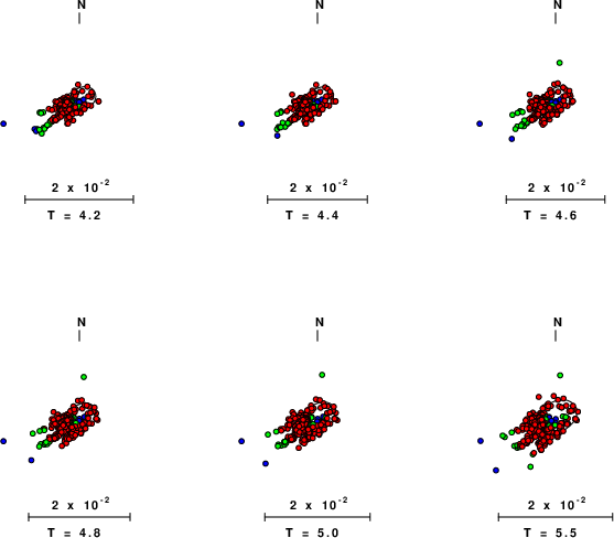
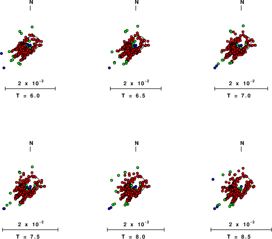
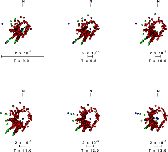
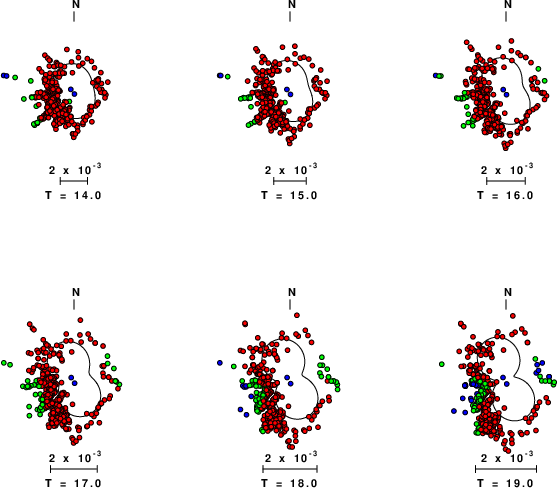
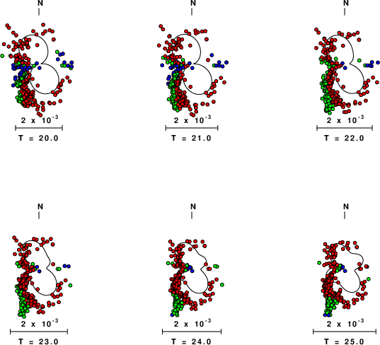
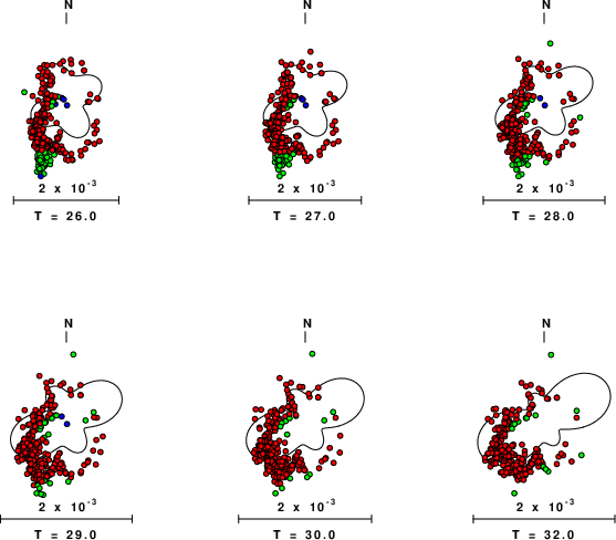
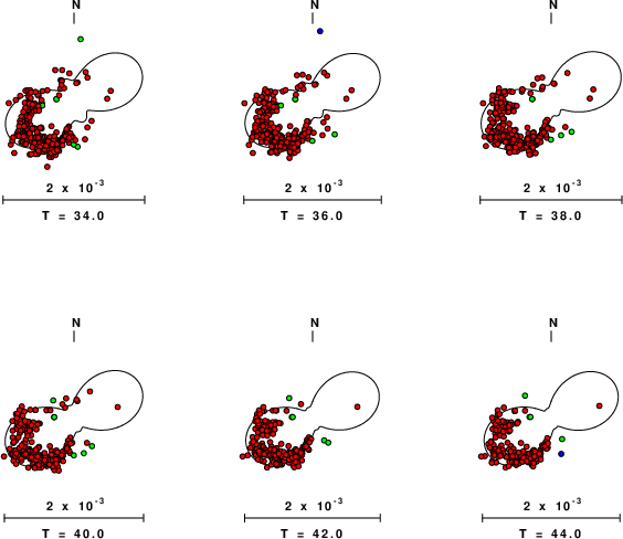
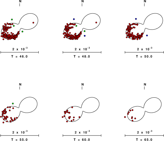
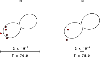
The next set of figures compares the observed and predicted surface wave radiation patterns as a function of period. The observed spectral amplitude have been corrected for anleastic attenuation by multiplication by a factor of eγr and corrected for surface wave geometrical spreading to a reference distance of 1000km. If the theoretical γ values are not perfect, then observations at large distance will plot as outliers.
Love-wave radiation patterns
Rayleigh-wave radiation patterns
