Location
Location ANSS
The ANSS event ID is ak0133b7hme1 and the event page is at
https://earthquake.usgs.gov/earthquakes/eventpage/ak0133b7hme1/executive.
2013/03/13 08:05:44 62.556 -151.230 84.4 4.8 Alaska
Focal Mechanism
 USGS/SLU Moment Tensor Solution
 ENS  2013/03/13 08:05:44:0  62.56 -151.23  84.4 4.8 Alaska

 Stations used:
   AK.BPAW AK.BWN AK.CAST AK.CCB AK.DHY AK.DOT AK.EYAK AK.HDA
   AK.KLU AK.KNK AK.MCK AK.MDM AK.MLY AK.NEA AK.PAX AK.PPD
   AK.PPLA AK.RC01 AK.RIDG AK.RND AK.SAW AK.SCM AK.SCRK AK.SWD
   AK.TRF AK.WRH AT.PMR AT.SVW2 IU.COLA

 Filtering commands used:
   hp c 0.02 n 3
   lp c 0.07 n 3

 Best Fitting Double Couple
  Mo = 1.32e+23 dyne-cm
  Mw = 4.68
  Z  = 91 km
  Plane   Strike  Dip  Rake
   NP1       60    60    55
   NP2      294    45   135
  Principal Axes:
   Axis    Value   Plunge  Azimuth
    T   1.32e+23     59     278
    N   0.00e+00     30      79
    P  -1.32e+23      9     174

 Moment Tensor: (dyne-cm)
    Component   Value
       Mxx    -1.27e+23
       Mxy     7.75e+21
       Mxz     2.79e+22
       Myy     3.33e+22
       Myz    -5.97e+22
       Mzz     9.35e+22


                     --------------
                 ----------------------
              ----------------------------
             ------------------------------
           -----############-----------------
          -######################-------------
         ###########################---------##
        ###############################------###
        #################################---####
       ############   ####################-######
       ############ T ###################---#####
       ############   #################------####
       ##############################---------###
        ###########################-----------##
        ########################---------------#
         ###################-------------------
          #############-----------------------
           ----------------------------------
             ------------------------------
              ----------------------------
                 -----------   --------
                     ------- P ----


 Global CMT Convention Moment Tensor:
      R          T          P
  9.35e+22   2.79e+22   5.97e+22
  2.79e+22  -1.27e+23  -7.75e+21
  5.97e+22  -7.75e+21   3.33e+22


Details of the solution is found at

http://www.eas.slu.edu/eqc/eqc_mt/MECH.NA/20130313080544/index.html
|
Preferred Solution
The preferred solution from an analysis of the surface-wave spectral amplitude radiation pattern, waveform inversion or first motion observations is
      STK = 60
      DIP = 60
     RAKE = 55
       MW = 4.68
       HS = 91.0
The NDK file is 20130313080544.ndk
The waveform inversion is preferred.
Magnitudes
Given the availability of digital waveforms for determination of the moment tensor, this section documents the added processing leading to mLg, if appropriate to the region, and ML by application of the respective IASPEI formulae. As a research study, the linear distance term of the IASPEI formula
for ML is adjusted to remove a linear distance trend in residuals to give a regionally defined ML. The defined ML uses horizontal component recordings, but the same procedure is applied to the vertical components since there may be some interest in vertical component ground motions. Residual plots versus distance may indicate interesting features of ground motion scaling in some distance ranges. A residual plot of the regionalized magnitude is given as a function of distance and azimuth, since data sets may transcend different wave propagation provinces.
ML Magnitude
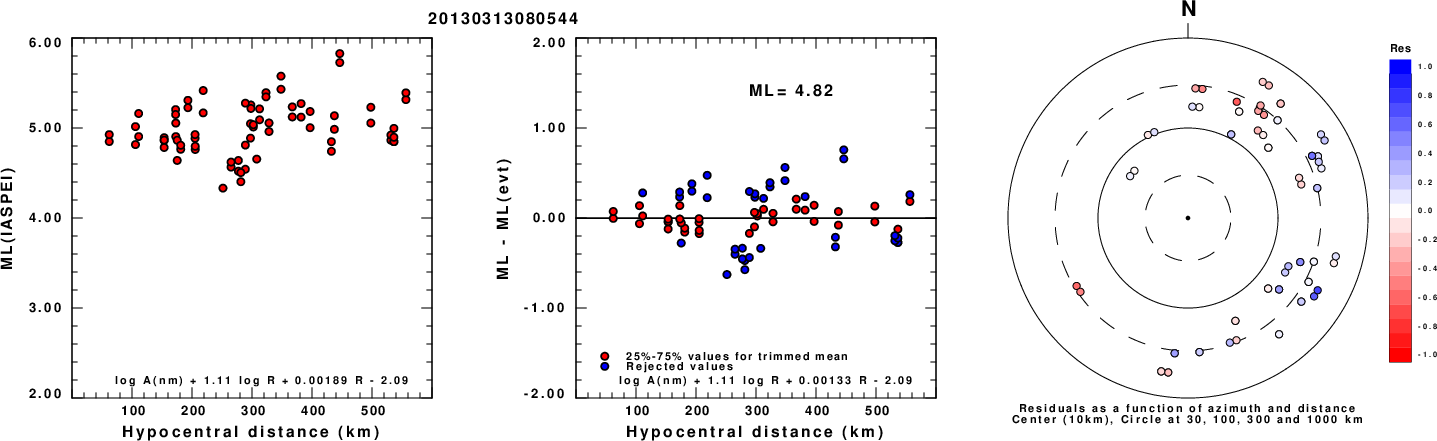
Left: ML computed using the IASPEI formula for Horizontal components. Center: ML residuals computed using a modified IASPEI formula that accounts for path specific attenuation; the values used for the trimmed mean are indicated. The ML relation used for each figure is given at the bottom of each plot.
Right: Residuals from new relation as a function of distance and azimuth.
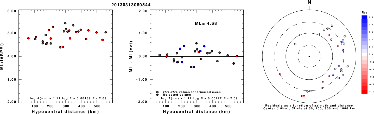
Left: ML computed using the IASPEI formula for Vertical components (research). Center: ML residuals computed using a modified IASPEI formula that accounts for path specific attenuation; the values used for the trimmed mean are indicated. The ML relation used for each figure is given at the bottom of each plot.
Right: Residuals from new relation as a function of distance and azimuth.
Context
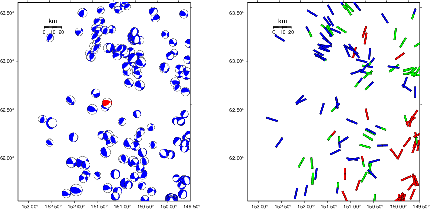
The left panel of the next figure presents the focal mechanism for this earthquake (red) in the context of other nearby events (blue) in the SLU Moment Tensor Catalog. The right panel shows the inferred direction of maximum compressive stress and the type of faulting (green is strike-slip, red is normal, blue is thrust; oblique is shown by a combination of colors). Thus context plot is useful for assessing the appropriateness of the moment tensor of this event.
Waveform Inversion using wvfgrd96
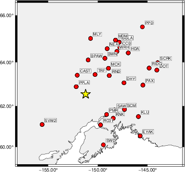
The focal mechanism was determined using broadband seismic waveforms. The location of the event (star) and the
stations used for (red) the waveform inversion are shown in the next figure.
|
|
Location of broadband stations used for waveform inversion
|
The program wvfgrd96 was used with good traces observed at short distance to determine the focal mechanism, depth and seismic moment. This technique requires a high quality signal and well determined velocity model for the Green's functions. To the extent that these are the quality data, this type of mechanism should be preferred over the radiation pattern technique which requires the separate step of defining the pressure and tension quadrants and the correct strike.
The observed and predicted traces are filtered using the following gsac commands:
hp c 0.02 n 3
lp c 0.07 n 3
The results of this grid search are as follow:
           DEPTH  STK   DIP  RAKE   MW    FIT
WVFGRD96    0.5    85    45   -75   3.73 0.2132
WVFGRD96    1.0    85    45   -75   3.77 0.2086
WVFGRD96    2.0    85    50   -80   3.88 0.2457
WVFGRD96    3.0    85    45   -75   3.93 0.2374
WVFGRD96    4.0    95    45   -60   3.93 0.2109
WVFGRD96    5.0    95    45   -55   3.93 0.2003
WVFGRD96    6.0    30    70   -45   3.91 0.2028
WVFGRD96    7.0    25    65   -45   3.93 0.2205
WVFGRD96    8.0    30    70   -50   3.99 0.2286
WVFGRD96    9.0    25    65   -50   4.01 0.2414
WVFGRD96   10.0    30    65   -45   4.01 0.2512
WVFGRD96   11.0   245    65    65   4.04 0.2596
WVFGRD96   12.0   240    65    60   4.04 0.2686
WVFGRD96   13.0   240    65    60   4.05 0.2757
WVFGRD96   14.0   240    65    60   4.06 0.2807
WVFGRD96   15.0   240    65    55   4.07 0.2842
WVFGRD96   16.0   235    65    50   4.08 0.2871
WVFGRD96   17.0   235    65    50   4.09 0.2901
WVFGRD96   18.0   235    65    50   4.10 0.2916
WVFGRD96   19.0   230    70    45   4.11 0.2941
WVFGRD96   20.0   230    70    45   4.12 0.2964
WVFGRD96   21.0   230    70    45   4.13 0.2983
WVFGRD96   22.0   230    70    45   4.14 0.3002
WVFGRD96   23.0   230    70    45   4.15 0.2987
WVFGRD96   24.0   230    70    40   4.16 0.2993
WVFGRD96   25.0   225    70    40   4.17 0.3006
WVFGRD96   26.0   225    70    40   4.17 0.2981
WVFGRD96   27.0   225    70    40   4.18 0.2986
WVFGRD96   28.0   225    70    40   4.19 0.2988
WVFGRD96   29.0   225    65    40   4.20 0.2966
WVFGRD96   30.0   225    65    40   4.21 0.2973
WVFGRD96   31.0   220    65    35   4.22 0.2959
WVFGRD96   32.0   215    60    30   4.23 0.2984
WVFGRD96   33.0   215    60    30   4.24 0.3012
WVFGRD96   34.0   215    60    30   4.25 0.3020
WVFGRD96   35.0   215    60    30   4.26 0.3044
WVFGRD96   36.0   215    60    30   4.27 0.3056
WVFGRD96   37.0    50    75    30   4.30 0.3077
WVFGRD96   38.0    50    75    25   4.33 0.3104
WVFGRD96   39.0    50    75    25   4.34 0.3133
WVFGRD96   40.0   220    60    40   4.38 0.3225
WVFGRD96   41.0   220    60    40   4.39 0.3250
WVFGRD96   42.0   220    60    40   4.40 0.3283
WVFGRD96   43.0   220    60    40   4.41 0.3324
WVFGRD96   44.0   220    60    40   4.42 0.3360
WVFGRD96   45.0   220    60    40   4.43 0.3400
WVFGRD96   46.0   220    60    40   4.44 0.3433
WVFGRD96   47.0   220    60    40   4.45 0.3465
WVFGRD96   48.0    50    65    35   4.48 0.3532
WVFGRD96   49.0    50    65    35   4.49 0.3598
WVFGRD96   50.0    50    65    35   4.50 0.3678
WVFGRD96   51.0    50    65    35   4.51 0.3754
WVFGRD96   52.0    50    65    35   4.52 0.3838
WVFGRD96   53.0    50    65    35   4.53 0.3923
WVFGRD96   54.0    50    65    35   4.54 0.4009
WVFGRD96   55.0    50    55    45   4.55 0.4117
WVFGRD96   56.0    50    55    45   4.56 0.4270
WVFGRD96   57.0    50    55    45   4.57 0.4427
WVFGRD96   58.0    50    55    45   4.57 0.4581
WVFGRD96   59.0    50    55    45   4.58 0.4731
WVFGRD96   60.0    50    55    45   4.59 0.4881
WVFGRD96   61.0    55    55    50   4.60 0.5023
WVFGRD96   62.0    55    55    50   4.60 0.5174
WVFGRD96   63.0    55    55    50   4.61 0.5321
WVFGRD96   64.0    55    55    50   4.61 0.5452
WVFGRD96   65.0    55    55    50   4.62 0.5586
WVFGRD96   66.0    55    55    50   4.62 0.5709
WVFGRD96   67.0    55    55    50   4.63 0.5841
WVFGRD96   68.0    55    55    50   4.63 0.5951
WVFGRD96   69.0    55    55    50   4.64 0.6060
WVFGRD96   70.0    55    55    50   4.64 0.6168
WVFGRD96   71.0    60    55    55   4.64 0.6263
WVFGRD96   72.0    60    55    55   4.65 0.6362
WVFGRD96   73.0    60    55    55   4.65 0.6450
WVFGRD96   74.0    60    55    55   4.65 0.6534
WVFGRD96   75.0    60    55    55   4.66 0.6607
WVFGRD96   76.0    60    55    55   4.66 0.6682
WVFGRD96   77.0    60    55    55   4.66 0.6738
WVFGRD96   78.0    60    55    55   4.66 0.6799
WVFGRD96   79.0    60    55    55   4.66 0.6845
WVFGRD96   80.0    60    55    55   4.66 0.6889
WVFGRD96   81.0    60    60    55   4.67 0.6942
WVFGRD96   82.0    60    60    55   4.67 0.6982
WVFGRD96   83.0    60    60    55   4.67 0.7022
WVFGRD96   84.0    60    60    55   4.67 0.7053
WVFGRD96   85.0    60    60    55   4.67 0.7080
WVFGRD96   86.0    60    60    55   4.67 0.7102
WVFGRD96   87.0    60    60    55   4.68 0.7118
WVFGRD96   88.0    60    60    55   4.68 0.7132
WVFGRD96   89.0    60    60    55   4.68 0.7144
WVFGRD96   90.0    60    60    55   4.68 0.7141
WVFGRD96   91.0    60    60    55   4.68 0.7147
WVFGRD96   92.0    60    60    55   4.68 0.7142
WVFGRD96   93.0    60    60    55   4.68 0.7139
WVFGRD96   94.0    60    60    55   4.67 0.7125
WVFGRD96   95.0    60    60    55   4.67 0.7119
WVFGRD96   96.0    65    60    60   4.68 0.7103
WVFGRD96   97.0    65    60    60   4.68 0.7092
WVFGRD96   98.0    65    60    60   4.68 0.7076
WVFGRD96   99.0    65    60    60   4.68 0.7065
The best solution is
WVFGRD96 91.0 60 60 55 4.68 0.7147
The mechanism corresponding to the best fit is
|
|
Figure 1. Waveform inversion focal mechanism
|
The best fit as a function of depth is given in the following figure:
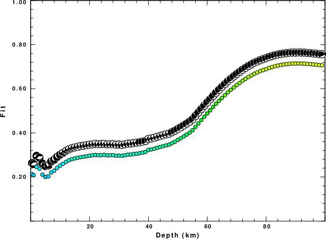
|
|
Figure 2. Depth sensitivity for waveform mechanism
|
The comparison of the observed and predicted waveforms is given in the next figure. The red traces are the observed and the blue are the predicted.
Each observed-predicted component is plotted to the same scale and peak amplitudes are indicated by the numbers to the left of each trace. A pair of numbers is given in black at the right of each predicted traces. The upper number it the time shift required for maximum correlation between the observed and predicted traces. This time shift is required because the synthetics are not computed at exactly the same distance as the observed, the velocity model used in the predictions may not be perfect and the epicentral parameters may be be off.
A positive time shift indicates that the prediction is too fast and should be delayed to match the observed trace (shift to the right in this figure). A negative value indicates that the prediction is too slow. The lower number gives the percentage of variance reduction to characterize the individual goodness of fit (100% indicates a perfect fit).
The bandpass filter used in the processing and for the display was
hp c 0.02 n 3
lp c 0.07 n 3
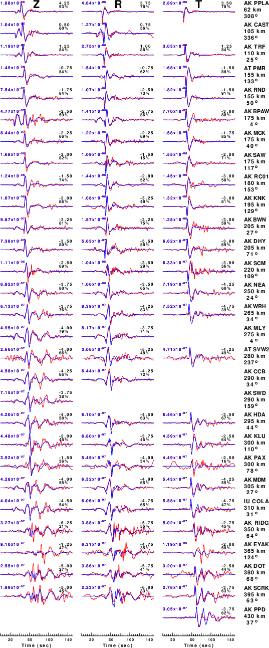
|
|
Figure 3. Waveform comparison for selected depth. Red: observed; Blue - predicted. The time shift with respect to the model prediction is indicated. The percent of fit is also indicated. The time scale is relative to the first trace sample.
|
|
|
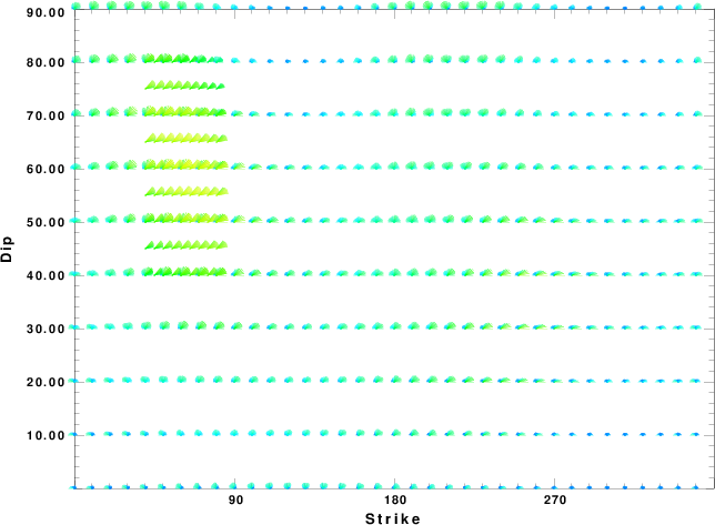
Focal mechanism sensitivity at the preferred depth. The red color indicates a very good fit to the waveforms.
Each solution is plotted as a vector at a given value of strike and dip with the angle of the vector representing the rake angle, measured, with respect to the upward vertical (N) in the figure.
|
A check on the assumed source location is possible by looking at the time shifts between the observed and predicted traces. The time shifts for waveform matching arise for several reasons:
- The origin time and epicentral distance are incorrect
- The velocity model used for the inversion is incorrect
- The velocity model used to define the P-arrival time is not the
same as the velocity model used for the waveform inversion
(assuming that the initial trace alignment is based on the
P arrival time)
Assuming only a mislocation, the time shifts are fit to a functional form:
Time_shift = A + B cos Azimuth + C Sin Azimuth
The time shifts for this inversion lead to the next figure:
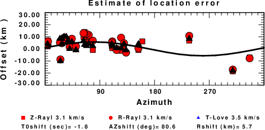
The derived shift in origin time and epicentral coordinates are given at the bottom of the figure.
Velocity Model
The WUS model used for the waveform synthetic seismograms and for the surface wave eigenfunctions and dispersion is as follows
(The format is in the model96 format of Computer Programs in Seismology).
MODEL.01
Model after     8 iterations
ISOTROPIC
KGS
FLAT EARTH
1-D
CONSTANT VELOCITY
LINE08
LINE09
LINE10
LINE11
      H(KM)   VP(KM/S)   VS(KM/S) RHO(GM/CC)         QP         QS       ETAP       ETAS      FREFP      FREFS
     1.9000     3.4065     2.0089     2.2150  0.302E-02  0.679E-02   0.00       0.00       1.00       1.00
     6.1000     5.5445     3.2953     2.6089  0.349E-02  0.784E-02   0.00       0.00       1.00       1.00
    13.0000     6.2708     3.7396     2.7812  0.212E-02  0.476E-02   0.00       0.00       1.00       1.00
    19.0000     6.4075     3.7680     2.8223  0.111E-02  0.249E-02   0.00       0.00       1.00       1.00
     0.0000     7.9000     4.6200     3.2760  0.164E-10  0.370E-10   0.00       0.00       1.00       1.00
Last Changed Fri Apr 26 04:48:02 PM CDT 2024