Location
Location ANSS
The ANSS event ID is ak01336gm5vh and the event page is at
https://earthquake.usgs.gov/earthquakes/eventpage/ak01336gm5vh/executive.
2013/03/10 21:05:18 61.542 -150.475 61.9 4.1 Alaska
Focal Mechanism
 USGS/SLU Moment Tensor Solution
 ENS  2013/03/10 21:05:18:0  61.54 -150.48  61.9 4.1 Alaska

 Stations used:
   AK.CAST AK.DIV AK.HIN AK.KNK AK.PPLA AK.RC01 AK.RIDG AK.SAW
   AK.SCM AK.SSN AK.SWD AT.MENT AT.PMR

 Filtering commands used:
   hp c 0.02 n 3
   lp c 0.06 n 3

 Best Fitting Double Couple
  Mo = 2.69e+22 dyne-cm
  Mw = 4.22
  Z  = 71 km
  Plane   Strike  Dip  Rake
   NP1      145    90   -155
   NP2       55    65     0
  Principal Axes:
   Axis    Value   Plunge  Azimuth
    T   2.69e+22     17     277
    N   0.00e+00     65     145
    P  -2.69e+22     17      13

 Moment Tensor: (dyne-cm)
    Component   Value
       Mxx    -2.29e+22
       Mxy    -8.34e+21
       Mxz    -6.52e+21
       Myy     2.29e+22
       Myz    -9.32e+21
       Mzz     0.00e+00


                     ---------   --
                 ------------- P ------
              ###-------------   ---------
             #####-------------------------
           #########-------------------------
          ###########------------------------#
         #############----------------------###
        ###############--------------------#####
        #   #############-----------------######
       ## T ##############--------------#########
       ##   ###############------------##########
       ######################--------############
       #######################-----##############
        #######################-################
        ######################---###############
         ##################-------#############
          ############-------------###########
           -##----------------------#########
             -------------------------#####
              -------------------------###
                 ----------------------
                     --------------


 Global CMT Convention Moment Tensor:
      R          T          P
  0.00e+00  -6.52e+21   9.32e+21
 -6.52e+21  -2.29e+22   8.34e+21
  9.32e+21   8.34e+21   2.29e+22


Details of the solution is found at

http://www.eas.slu.edu/eqc/eqc_mt/MECH.NA/20130310210518/index.html
|
Preferred Solution
The preferred solution from an analysis of the surface-wave spectral amplitude radiation pattern, waveform inversion or first motion observations is
      STK = 55
      DIP = 65
     RAKE = 0
       MW = 4.22
       HS = 71.0
The NDK file is 20130310210518.ndk
The waveform inversion is preferred.
Magnitudes
Given the availability of digital waveforms for determination of the moment tensor, this section documents the added processing leading to mLg, if appropriate to the region, and ML by application of the respective IASPEI formulae. As a research study, the linear distance term of the IASPEI formula
for ML is adjusted to remove a linear distance trend in residuals to give a regionally defined ML. The defined ML uses horizontal component recordings, but the same procedure is applied to the vertical components since there may be some interest in vertical component ground motions. Residual plots versus distance may indicate interesting features of ground motion scaling in some distance ranges. A residual plot of the regionalized magnitude is given as a function of distance and azimuth, since data sets may transcend different wave propagation provinces.
ML Magnitude
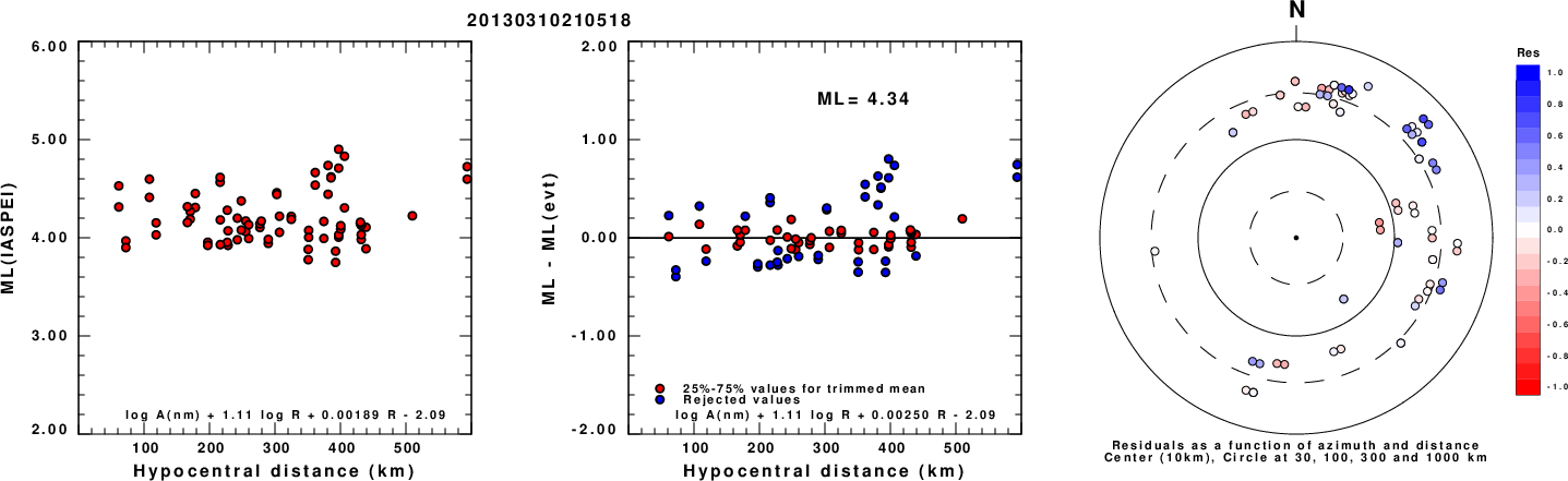
Left: ML computed using the IASPEI formula for Horizontal components. Center: ML residuals computed using a modified IASPEI formula that accounts for path specific attenuation; the values used for the trimmed mean are indicated. The ML relation used for each figure is given at the bottom of each plot.
Right: Residuals from new relation as a function of distance and azimuth.
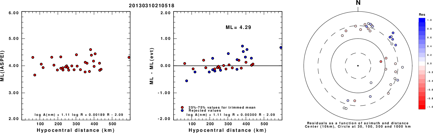
Left: ML computed using the IASPEI formula for Vertical components (research). Center: ML residuals computed using a modified IASPEI formula that accounts for path specific attenuation; the values used for the trimmed mean are indicated. The ML relation used for each figure is given at the bottom of each plot.
Right: Residuals from new relation as a function of distance and azimuth.
Context
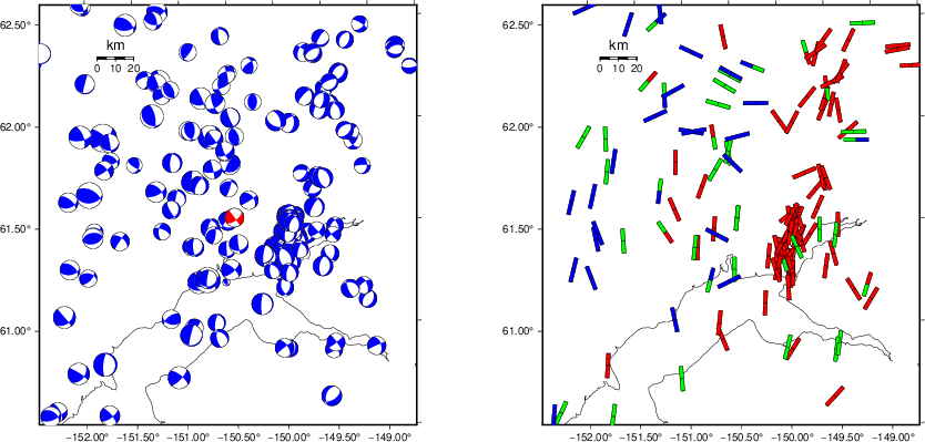
The left panel of the next figure presents the focal mechanism for this earthquake (red) in the context of other nearby events (blue) in the SLU Moment Tensor Catalog. The right panel shows the inferred direction of maximum compressive stress and the type of faulting (green is strike-slip, red is normal, blue is thrust; oblique is shown by a combination of colors). Thus context plot is useful for assessing the appropriateness of the moment tensor of this event.
Waveform Inversion using wvfgrd96
The focal mechanism was determined using broadband seismic waveforms. The location of the event (star) and the
stations used for (red) the waveform inversion are shown in the next figure.

|
|
Location of broadband stations used for waveform inversion
|
The program wvfgrd96 was used with good traces observed at short distance to determine the focal mechanism, depth and seismic moment. This technique requires a high quality signal and well determined velocity model for the Green's functions. To the extent that these are the quality data, this type of mechanism should be preferred over the radiation pattern technique which requires the separate step of defining the pressure and tension quadrants and the correct strike.
The observed and predicted traces are filtered using the following gsac commands:
hp c 0.02 n 3
lp c 0.06 n 3
The results of this grid search are as follow:
           DEPTH  STK   DIP  RAKE   MW    FIT
WVFGRD96    0.5    50    55   -15   3.24 0.1165
WVFGRD96    1.0    50    60   -10   3.28 0.1303
WVFGRD96    2.0    55    55     0   3.42 0.1849
WVFGRD96    3.0    55    55     5   3.49 0.2140
WVFGRD96    4.0    55    60    20   3.55 0.2416
WVFGRD96    5.0    55    65    20   3.57 0.2678
WVFGRD96    6.0    55    65    20   3.60 0.2877
WVFGRD96    7.0    50    70    15   3.63 0.3107
WVFGRD96    8.0    50    65    15   3.68 0.3341
WVFGRD96    9.0    50    65    15   3.70 0.3534
WVFGRD96   10.0    50    70    15   3.72 0.3702
WVFGRD96   11.0    50    70    15   3.73 0.3818
WVFGRD96   12.0    50    70    10   3.74 0.3943
WVFGRD96   13.0    50    70    10   3.76 0.4045
WVFGRD96   14.0    50    75    10   3.77 0.4131
WVFGRD96   15.0    50    75    10   3.78 0.4226
WVFGRD96   16.0    50    75    10   3.79 0.4309
WVFGRD96   17.0    50    75     5   3.80 0.4364
WVFGRD96   18.0    50    80    10   3.81 0.4440
WVFGRD96   19.0    50    80    10   3.82 0.4495
WVFGRD96   20.0    50    80     5   3.83 0.4569
WVFGRD96   21.0    55    80    10   3.83 0.4621
WVFGRD96   22.0    55    80    10   3.84 0.4684
WVFGRD96   23.0    55    80    10   3.85 0.4732
WVFGRD96   24.0    55    80    10   3.86 0.4791
WVFGRD96   25.0    55    80     5   3.87 0.4843
WVFGRD96   26.0    55    80     5   3.88 0.4903
WVFGRD96   27.0    55    80     5   3.89 0.4951
WVFGRD96   28.0    55    80     5   3.90 0.5005
WVFGRD96   29.0    55    80     5   3.90 0.5064
WVFGRD96   30.0    55    80     5   3.91 0.5120
WVFGRD96   31.0    50    85     5   3.93 0.5179
WVFGRD96   32.0    50    85     5   3.94 0.5233
WVFGRD96   33.0    50    85     5   3.96 0.5290
WVFGRD96   34.0    50    85     5   3.97 0.5347
WVFGRD96   35.0    50    85     5   3.98 0.5393
WVFGRD96   36.0    50    85     0   3.99 0.5432
WVFGRD96   37.0    50    85     0   4.01 0.5488
WVFGRD96   38.0    50    85     0   4.02 0.5545
WVFGRD96   39.0    50    85     0   4.04 0.5597
WVFGRD96   40.0    50    80     0   4.06 0.5663
WVFGRD96   41.0    50    80     0   4.07 0.5696
WVFGRD96   42.0    50    80     0   4.08 0.5717
WVFGRD96   43.0    50    80     0   4.09 0.5734
WVFGRD96   44.0    50    80     0   4.10 0.5763
WVFGRD96   45.0    50    80     0   4.10 0.5785
WVFGRD96   46.0    50    80     0   4.11 0.5797
WVFGRD96   47.0    50    80     0   4.12 0.5825
WVFGRD96   48.0    50    80     0   4.13 0.5844
WVFGRD96   49.0    50    80     0   4.13 0.5850
WVFGRD96   50.0    50    80     0   4.14 0.5875
WVFGRD96   51.0    50    80     0   4.15 0.5887
WVFGRD96   52.0    50    80     0   4.15 0.5895
WVFGRD96   53.0    50    80     0   4.16 0.5912
WVFGRD96   54.0    50    80     0   4.16 0.5913
WVFGRD96   55.0    50    80     0   4.17 0.5928
WVFGRD96   56.0    50    75     0   4.17 0.5931
WVFGRD96   57.0    50    75     0   4.17 0.5942
WVFGRD96   58.0    50    75     0   4.18 0.5949
WVFGRD96   59.0    50    75     5   4.18 0.5958
WVFGRD96   60.0    50    75     5   4.19 0.5969
WVFGRD96   61.0    50    75     5   4.19 0.5976
WVFGRD96   62.0    50    75     5   4.20 0.5986
WVFGRD96   63.0    50    75     5   4.20 0.5987
WVFGRD96   64.0    50    75     5   4.21 0.5994
WVFGRD96   65.0    50    75     5   4.21 0.5990
WVFGRD96   66.0    55    65     0   4.20 0.5997
WVFGRD96   67.0    55    65     0   4.20 0.6000
WVFGRD96   68.0    55    65     0   4.21 0.6003
WVFGRD96   69.0    55    65     0   4.21 0.6004
WVFGRD96   70.0    55    65     0   4.21 0.6000
WVFGRD96   71.0    55    65     0   4.22 0.6004
WVFGRD96   72.0    55    65     0   4.22 0.5989
WVFGRD96   73.0    55    65     0   4.22 0.5992
WVFGRD96   74.0    55    65     0   4.23 0.5982
WVFGRD96   75.0    55    65     5   4.23 0.5974
WVFGRD96   76.0    55    65     5   4.23 0.5966
WVFGRD96   77.0    55    65     5   4.24 0.5954
WVFGRD96   78.0    55    65     5   4.24 0.5954
WVFGRD96   79.0    55    65     5   4.24 0.5936
WVFGRD96   80.0    55    65     5   4.25 0.5928
WVFGRD96   81.0    55    65     5   4.25 0.5916
WVFGRD96   82.0    55    65     5   4.25 0.5889
WVFGRD96   83.0    55    65     5   4.25 0.5886
WVFGRD96   84.0    55    65    10   4.26 0.5865
WVFGRD96   85.0    55    65    10   4.26 0.5846
WVFGRD96   86.0    55    65    10   4.26 0.5839
WVFGRD96   87.0    55    65    10   4.26 0.5815
WVFGRD96   88.0    55    65    10   4.27 0.5798
WVFGRD96   89.0    55    65    10   4.27 0.5784
WVFGRD96   90.0    55    65    10   4.27 0.5758
WVFGRD96   91.0    55    65    10   4.27 0.5740
WVFGRD96   92.0    55    65    10   4.28 0.5720
WVFGRD96   93.0    55    65    10   4.28 0.5693
WVFGRD96   94.0    55    65    15   4.28 0.5670
WVFGRD96   95.0    55    65    15   4.28 0.5655
WVFGRD96   96.0    55    65    15   4.28 0.5628
WVFGRD96   97.0    55    65    15   4.29 0.5607
WVFGRD96   98.0    55    65    15   4.29 0.5588
WVFGRD96   99.0    55    65    15   4.29 0.5564
The best solution is
WVFGRD96 71.0 55 65 0 4.22 0.6004
The mechanism corresponding to the best fit is
|
|
Figure 1. Waveform inversion focal mechanism
|
The best fit as a function of depth is given in the following figure:
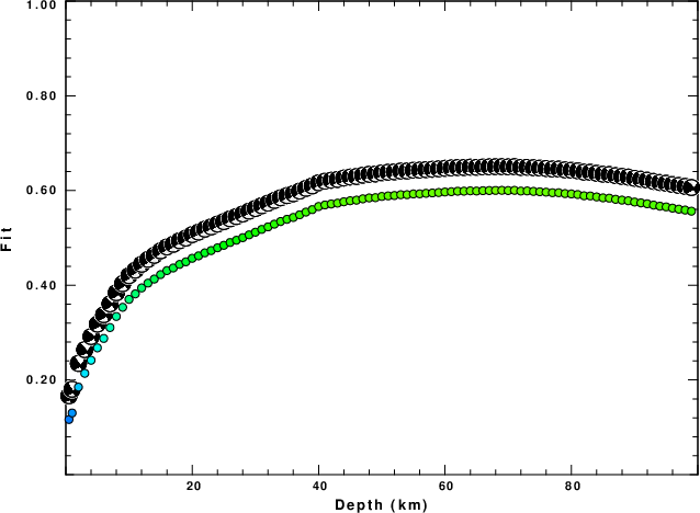
|
|
Figure 2. Depth sensitivity for waveform mechanism
|
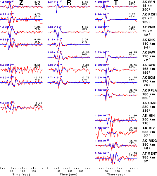
The comparison of the observed and predicted waveforms is given in the next figure. The red traces are the observed and the blue are the predicted.
Each observed-predicted component is plotted to the same scale and peak amplitudes are indicated by the numbers to the left of each trace. A pair of numbers is given in black at the right of each predicted traces. The upper number it the time shift required for maximum correlation between the observed and predicted traces. This time shift is required because the synthetics are not computed at exactly the same distance as the observed, the velocity model used in the predictions may not be perfect and the epicentral parameters may be be off.
A positive time shift indicates that the prediction is too fast and should be delayed to match the observed trace (shift to the right in this figure). A negative value indicates that the prediction is too slow. The lower number gives the percentage of variance reduction to characterize the individual goodness of fit (100% indicates a perfect fit).
The bandpass filter used in the processing and for the display was
hp c 0.02 n 3
lp c 0.06 n 3
|
|
Figure 3. Waveform comparison for selected depth. Red: observed; Blue - predicted. The time shift with respect to the model prediction is indicated. The percent of fit is also indicated. The time scale is relative to the first trace sample.
|
|
|
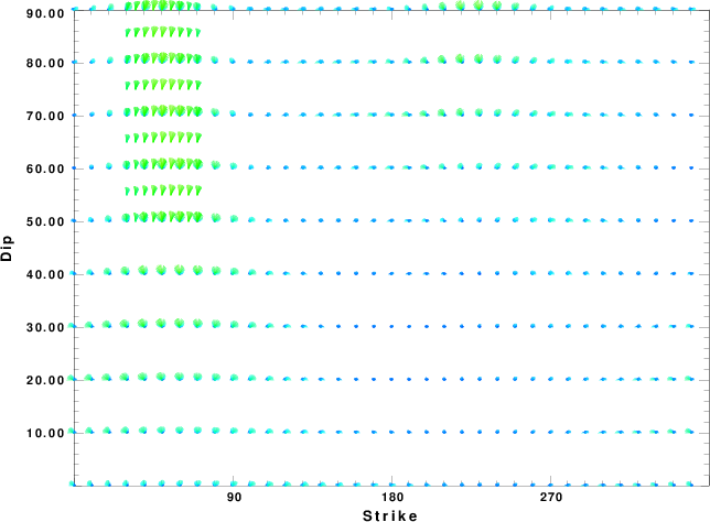
Focal mechanism sensitivity at the preferred depth. The red color indicates a very good fit to the waveforms.
Each solution is plotted as a vector at a given value of strike and dip with the angle of the vector representing the rake angle, measured, with respect to the upward vertical (N) in the figure.
|
A check on the assumed source location is possible by looking at the time shifts between the observed and predicted traces. The time shifts for waveform matching arise for several reasons:
- The origin time and epicentral distance are incorrect
- The velocity model used for the inversion is incorrect
- The velocity model used to define the P-arrival time is not the
same as the velocity model used for the waveform inversion
(assuming that the initial trace alignment is based on the
P arrival time)
Assuming only a mislocation, the time shifts are fit to a functional form:
Time_shift = A + B cos Azimuth + C Sin Azimuth
The time shifts for this inversion lead to the next figure:
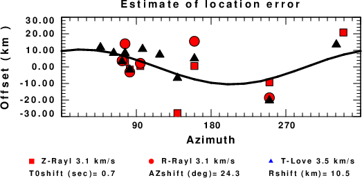
The derived shift in origin time and epicentral coordinates are given at the bottom of the figure.
Velocity Model
The WUS.model used for the waveform synthetic seismograms and for the surface wave eigenfunctions and dispersion is as follows
(The format is in the model96 format of Computer Programs in Seismology).
MODEL.01
Model after     8 iterations
ISOTROPIC
KGS
FLAT EARTH
1-D
CONSTANT VELOCITY
LINE08
LINE09
LINE10
LINE11
      H(KM)   VP(KM/S)   VS(KM/S) RHO(GM/CC)         QP         QS       ETAP       ETAS      FREFP      FREFS
     1.9000     3.4065     2.0089     2.2150  0.302E-02  0.679E-02   0.00       0.00       1.00       1.00
     6.1000     5.5445     3.2953     2.6089  0.349E-02  0.784E-02   0.00       0.00       1.00       1.00
    13.0000     6.2708     3.7396     2.7812  0.212E-02  0.476E-02   0.00       0.00       1.00       1.00
    19.0000     6.4075     3.7680     2.8223  0.111E-02  0.249E-02   0.00       0.00       1.00       1.00
     0.0000     7.9000     4.6200     3.2760  0.164E-10  0.370E-10   0.00       0.00       1.00       1.00
Last Changed Fri Apr 26 04:30:17 PM CDT 2024