Location
Location ANSS
The ANSS event ID is ak012gi080jr and the event page is at
https://earthquake.usgs.gov/earthquakes/eventpage/ak012gi080jr/executive.
2012/12/24 17:28:25 61.243 -150.764 64.4 4.4 Alaska
Focal Mechanism
 USGS/SLU Moment Tensor Solution
 ENS  2012/12/24 17:28:25:0  61.24 -150.76  64.4 4.4 Alaska

 Stations used:
   AK.GHO AK.KNK AK.PPLA AK.SAW AK.SCM AK.SKN AK.SSN AK.SWD
   AT.PMR

 Filtering commands used:
   hp c 0.02 n 3
   lp c 0.10 n 3

 Best Fitting Double Couple
  Mo = 2.43e+22 dyne-cm
  Mw = 4.19
  Z  = 70 km
  Plane   Strike  Dip  Rake
   NP1      188    82   -114
   NP2       80    25   -20
  Principal Axes:
   Axis    Value   Plunge  Azimuth
    T   2.43e+22     33     298
    N   0.00e+00     23     192
    P  -2.43e+22     48      73

 Moment Tensor: (dyne-cm)
    Component   Value
       Mxx     2.87e+21
       Mxy    -1.01e+22
       Mxz     1.67e+21
       Myy     3.49e+21
       Myz    -2.13e+22
       Mzz    -6.36e+21


                     #########-----
                 #############---------
              ###############-------------
             ################--------------
           #################-----------------
          ##################------------------
         #####   ##########--------------------
        ###### T ##########---------------------
        ######   ##########---------   ---------
       ###################---------- P ---------#
       ###################----------   ---------#
       ###################----------------------#
       ##################----------------------##
        #################---------------------##
        -################--------------------###
         -###############-------------------###
          --#############-----------------####
           ---###########--------------######
             -----#######-----------#######
              ----------#----#############
                 --------##############
                     ----##########


 Global CMT Convention Moment Tensor:
      R          T          P
 -6.36e+21   1.67e+21   2.13e+22
  1.67e+21   2.87e+21   1.01e+22
  2.13e+22   1.01e+22   3.49e+21


Details of the solution is found at

http://www.eas.slu.edu/eqc/eqc_mt/MECH.NA/20121224172825/index.html
|
Preferred Solution
The preferred solution from an analysis of the surface-wave spectral amplitude radiation pattern, waveform inversion or first motion observations is
      STK = 80
      DIP = 25
     RAKE = -20
       MW = 4.19
       HS = 70.0
The NDK file is 20121224172825.ndk
The waveform inversion is preferred.
Magnitudes
Given the availability of digital waveforms for determination of the moment tensor, this section documents the added processing leading to mLg, if appropriate to the region, and ML by application of the respective IASPEI formulae. As a research study, the linear distance term of the IASPEI formula
for ML is adjusted to remove a linear distance trend in residuals to give a regionally defined ML. The defined ML uses horizontal component recordings, but the same procedure is applied to the vertical components since there may be some interest in vertical component ground motions. Residual plots versus distance may indicate interesting features of ground motion scaling in some distance ranges. A residual plot of the regionalized magnitude is given as a function of distance and azimuth, since data sets may transcend different wave propagation provinces.
ML Magnitude
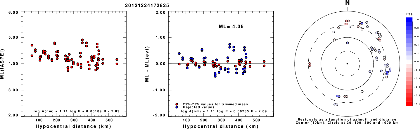
Left: ML computed using the IASPEI formula for Horizontal components. Center: ML residuals computed using a modified IASPEI formula that accounts for path specific attenuation; the values used for the trimmed mean are indicated. The ML relation used for each figure is given at the bottom of each plot.
Right: Residuals from new relation as a function of distance and azimuth.
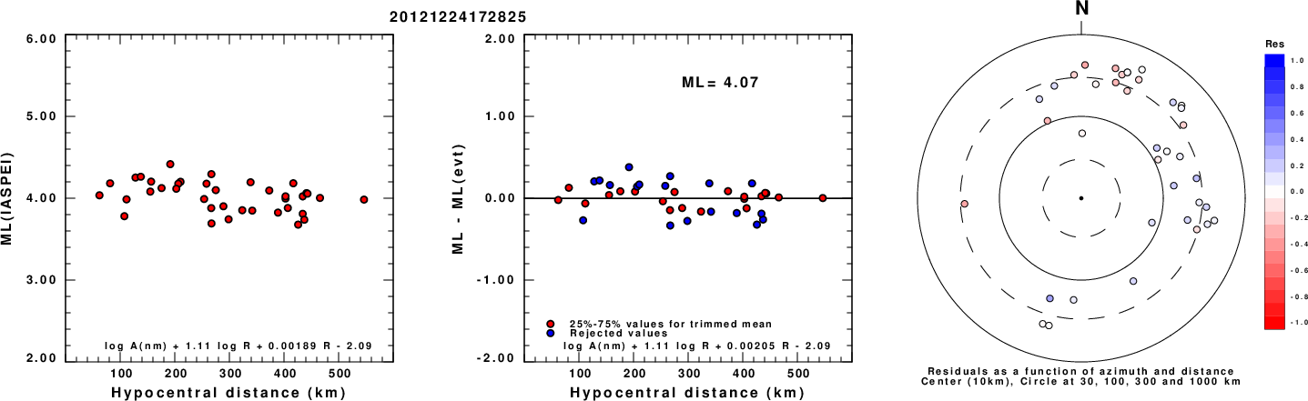
Left: ML computed using the IASPEI formula for Vertical components (research). Center: ML residuals computed using a modified IASPEI formula that accounts for path specific attenuation; the values used for the trimmed mean are indicated. The ML relation used for each figure is given at the bottom of each plot.
Right: Residuals from new relation as a function of distance and azimuth.
Context
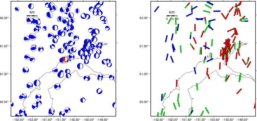
The left panel of the next figure presents the focal mechanism for this earthquake (red) in the context of other nearby events (blue) in the SLU Moment Tensor Catalog. The right panel shows the inferred direction of maximum compressive stress and the type of faulting (green is strike-slip, red is normal, blue is thrust; oblique is shown by a combination of colors). Thus context plot is useful for assessing the appropriateness of the moment tensor of this event.
Waveform Inversion using wvfgrd96
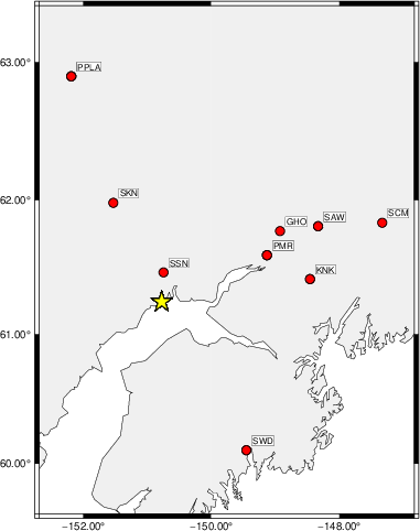
The focal mechanism was determined using broadband seismic waveforms. The location of the event (star) and the
stations used for (red) the waveform inversion are shown in the next figure.
|
|
Location of broadband stations used for waveform inversion
|
The program wvfgrd96 was used with good traces observed at short distance to determine the focal mechanism, depth and seismic moment. This technique requires a high quality signal and well determined velocity model for the Green's functions. To the extent that these are the quality data, this type of mechanism should be preferred over the radiation pattern technique which requires the separate step of defining the pressure and tension quadrants and the correct strike.
The observed and predicted traces are filtered using the following gsac commands:
hp c 0.02 n 3
lp c 0.10 n 3
The results of this grid search are as follow:
           DEPTH  STK   DIP  RAKE   MW    FIT
WVFGRD96    0.5    35    40   -90   3.23 0.2152
WVFGRD96    1.0    30    80    10   3.22 0.2190
WVFGRD96    2.0     5    75   -15   3.30 0.2817
WVFGRD96    3.0    25    90     5   3.45 0.3114
WVFGRD96    4.0   205    85   -10   3.51 0.3144
WVFGRD96    5.0   190    60    20   3.46 0.3323
WVFGRD96    6.0   190    60    20   3.50 0.3575
WVFGRD96    7.0    10    60    15   3.54 0.3818
WVFGRD96    8.0    10    55    20   3.59 0.4057
WVFGRD96    9.0   190    80    30   3.62 0.4172
WVFGRD96   10.0   185    90    30   3.63 0.4307
WVFGRD96   11.0   185    90    25   3.66 0.4386
WVFGRD96   12.0   185    85    25   3.67 0.4419
WVFGRD96   13.0   185    85    25   3.69 0.4422
WVFGRD96   14.0   185    85    25   3.71 0.4416
WVFGRD96   15.0   185    70    20   3.71 0.4366
WVFGRD96   16.0   185    75    20   3.73 0.4323
WVFGRD96   17.0   185    75    20   3.74 0.4261
WVFGRD96   18.0   185    75    20   3.76 0.4176
WVFGRD96   19.0   190    70    20   3.78 0.4096
WVFGRD96   20.0   190    70    20   3.79 0.4001
WVFGRD96   21.0   190    70    20   3.80 0.3906
WVFGRD96   22.0   190    70    15   3.81 0.3800
WVFGRD96   23.0   190    70    15   3.82 0.3659
WVFGRD96   24.0   190    70    15   3.82 0.3550
WVFGRD96   25.0   190    65    15   3.83 0.3436
WVFGRD96   26.0    30    85    10   3.87 0.3460
WVFGRD96   27.0    35    85    20   3.87 0.3561
WVFGRD96   28.0    35    85    20   3.88 0.3651
WVFGRD96   29.0    35    85    20   3.89 0.3717
WVFGRD96   30.0    35    85    25   3.89 0.3796
WVFGRD96   31.0    45    70    25   3.90 0.3884
WVFGRD96   32.0    45    70    25   3.91 0.3989
WVFGRD96   33.0    45    70    25   3.92 0.4078
WVFGRD96   34.0    45    70    25   3.93 0.4181
WVFGRD96   35.0    45    70    25   3.94 0.4289
WVFGRD96   36.0    45    70    25   3.95 0.4389
WVFGRD96   37.0    45    85    40   3.96 0.4479
WVFGRD96   38.0    45    85    40   3.96 0.4585
WVFGRD96   39.0    50    80    40   3.97 0.4669
WVFGRD96   40.0    45    85    55   4.06 0.4679
WVFGRD96   41.0    45    85    55   4.07 0.4760
WVFGRD96   42.0    45    85    55   4.08 0.4787
WVFGRD96   43.0    45    80    50   4.08 0.4858
WVFGRD96   44.0    50    75    45   4.09 0.4905
WVFGRD96   45.0    50    75    45   4.10 0.4963
WVFGRD96   46.0    65    25   -30   4.09 0.5050
WVFGRD96   47.0    65    25   -30   4.09 0.5148
WVFGRD96   48.0    70    25   -30   4.10 0.5234
WVFGRD96   49.0    70    25   -30   4.11 0.5338
WVFGRD96   50.0    70    25   -30   4.12 0.5439
WVFGRD96   51.0    70    25   -30   4.12 0.5519
WVFGRD96   52.0    70    25   -30   4.13 0.5595
WVFGRD96   53.0    70    25   -30   4.13 0.5683
WVFGRD96   54.0    75    25   -25   4.13 0.5747
WVFGRD96   55.0    75    25   -25   4.14 0.5799
WVFGRD96   56.0    75    25   -25   4.14 0.5876
WVFGRD96   57.0    75    25   -25   4.15 0.5945
WVFGRD96   58.0    75    25   -25   4.15 0.5989
WVFGRD96   59.0    75    25   -25   4.15 0.6011
WVFGRD96   60.0    75    25   -25   4.16 0.6070
WVFGRD96   61.0    75    25   -25   4.16 0.6109
WVFGRD96   62.0    75    25   -25   4.16 0.6131
WVFGRD96   63.0    75    25   -25   4.17 0.6148
WVFGRD96   64.0    80    25   -20   4.17 0.6191
WVFGRD96   65.0    80    25   -20   4.17 0.6206
WVFGRD96   66.0    80    25   -20   4.17 0.6217
WVFGRD96   67.0    80    25   -20   4.18 0.6232
WVFGRD96   68.0    80    25   -20   4.18 0.6235
WVFGRD96   69.0    80    25   -20   4.18 0.6255
WVFGRD96   70.0    80    25   -20   4.19 0.6257
WVFGRD96   71.0    85    25   -15   4.18 0.6240
WVFGRD96   72.0    85    25   -15   4.19 0.6243
WVFGRD96   73.0    85    25   -15   4.19 0.6247
WVFGRD96   74.0    85    25   -15   4.19 0.6247
WVFGRD96   75.0    90    25   -15   4.20 0.6249
WVFGRD96   76.0    90    25   -15   4.20 0.6217
WVFGRD96   77.0    90    25   -15   4.21 0.6211
WVFGRD96   78.0    90    20   -15   4.20 0.6208
WVFGRD96   79.0    90    20   -15   4.21 0.6215
WVFGRD96   80.0    95    25   -10   4.21 0.6189
WVFGRD96   81.0    95    20   -10   4.21 0.6175
WVFGRD96   82.0    95    20   -10   4.21 0.6151
WVFGRD96   83.0    95    20   -10   4.22 0.6153
WVFGRD96   84.0    95    20   -10   4.22 0.6147
WVFGRD96   85.0    95    20   -10   4.22 0.6123
WVFGRD96   86.0   100    25    -5   4.22 0.6102
WVFGRD96   87.0   100    25    -5   4.23 0.6072
WVFGRD96   88.0   100    25    -5   4.23 0.6066
WVFGRD96   89.0   100    25    -5   4.23 0.6061
WVFGRD96   90.0   105    25    -5   4.24 0.6037
WVFGRD96   91.0   105    25    -5   4.24 0.6019
WVFGRD96   92.0   105    25    -5   4.25 0.5978
WVFGRD96   93.0   105    25    -5   4.25 0.5966
WVFGRD96   94.0   110    25     0   4.25 0.5954
WVFGRD96   95.0   110    25     0   4.25 0.5946
WVFGRD96   96.0   110    25     0   4.25 0.5928
WVFGRD96   97.0   110    25     0   4.26 0.5907
WVFGRD96   98.0   110    25     0   4.26 0.5874
WVFGRD96   99.0   110    25     0   4.26 0.5872
The best solution is
WVFGRD96 70.0 80 25 -20 4.19 0.6257
The mechanism corresponding to the best fit is
|
|
Figure 1. Waveform inversion focal mechanism
|
The best fit as a function of depth is given in the following figure:
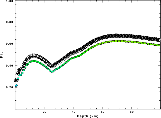
|
|
Figure 2. Depth sensitivity for waveform mechanism
|
The comparison of the observed and predicted waveforms is given in the next figure. The red traces are the observed and the blue are the predicted.
Each observed-predicted component is plotted to the same scale and peak amplitudes are indicated by the numbers to the left of each trace. A pair of numbers is given in black at the right of each predicted traces. The upper number it the time shift required for maximum correlation between the observed and predicted traces. This time shift is required because the synthetics are not computed at exactly the same distance as the observed, the velocity model used in the predictions may not be perfect and the epicentral parameters may be be off.
A positive time shift indicates that the prediction is too fast and should be delayed to match the observed trace (shift to the right in this figure). A negative value indicates that the prediction is too slow. The lower number gives the percentage of variance reduction to characterize the individual goodness of fit (100% indicates a perfect fit).
The bandpass filter used in the processing and for the display was
hp c 0.02 n 3
lp c 0.10 n 3
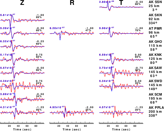
|
|
Figure 3. Waveform comparison for selected depth. Red: observed; Blue - predicted. The time shift with respect to the model prediction is indicated. The percent of fit is also indicated. The time scale is relative to the first trace sample.
|
|
|
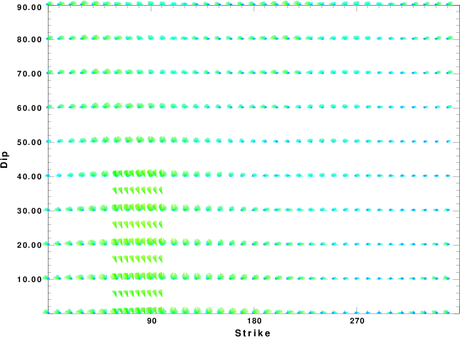
Focal mechanism sensitivity at the preferred depth. The red color indicates a very good fit to the waveforms.
Each solution is plotted as a vector at a given value of strike and dip with the angle of the vector representing the rake angle, measured, with respect to the upward vertical (N) in the figure.
|
A check on the assumed source location is possible by looking at the time shifts between the observed and predicted traces. The time shifts for waveform matching arise for several reasons:
- The origin time and epicentral distance are incorrect
- The velocity model used for the inversion is incorrect
- The velocity model used to define the P-arrival time is not the
same as the velocity model used for the waveform inversion
(assuming that the initial trace alignment is based on the
P arrival time)
Assuming only a mislocation, the time shifts are fit to a functional form:
Time_shift = A + B cos Azimuth + C Sin Azimuth
The time shifts for this inversion lead to the next figure:
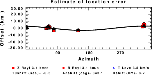
The derived shift in origin time and epicentral coordinates are given at the bottom of the figure.
Velocity Model
The WUS.model used for the waveform synthetic seismograms and for the surface wave eigenfunctions and dispersion is as follows
(The format is in the model96 format of Computer Programs in Seismology).
MODEL.01
Model after     8 iterations
ISOTROPIC
KGS
FLAT EARTH
1-D
CONSTANT VELOCITY
LINE08
LINE09
LINE10
LINE11
      H(KM)   VP(KM/S)   VS(KM/S) RHO(GM/CC)         QP         QS       ETAP       ETAS      FREFP      FREFS
     1.9000     3.4065     2.0089     2.2150  0.302E-02  0.679E-02   0.00       0.00       1.00       1.00
     6.1000     5.5445     3.2953     2.6089  0.349E-02  0.784E-02   0.00       0.00       1.00       1.00
    13.0000     6.2708     3.7396     2.7812  0.212E-02  0.476E-02   0.00       0.00       1.00       1.00
    19.0000     6.4075     3.7680     2.8223  0.111E-02  0.249E-02   0.00       0.00       1.00       1.00
     0.0000     7.9000     4.6200     3.2760  0.164E-10  0.370E-10   0.00       0.00       1.00       1.00
Last Changed Sat Apr 27 12:53:20 AM CDT 2024