Location
Location ANSS
The ANSS event ID is ak012fko16th and the event page is at
https://earthquake.usgs.gov/earthquakes/eventpage/ak012fko16th/executive.
2012/12/04 01:42:48 61.240 -150.768 63.7 5.8 Alaska
Focal Mechanism
 USGS/SLU Moment Tensor Solution
 ENS  2012/12/04 01:42:48:0  61.24 -150.77  63.7 5.8 Alaska

 Stations used:
   AK.BMR AK.BPAW AK.BRLK AK.CAST AK.CCB AK.CNP AK.DHY AK.DIV
   AK.DOT AK.EYAK AK.FID AK.GHO AK.GLI AK.GLM AK.HMT AK.HOM
   AK.KLU AK.KNK AK.MCK AK.MDM AK.PAX AK.PIN AK.PPD AK.PPLA
   AK.RAG AK.RC01 AK.RND AK.SAW AK.SCM AK.SKN AK.SWD AK.TRF
   AT.MID AT.PMR AT.SVW2 IU.COLA

 Filtering commands used:
   hp c 0.02 n 3
   lp c 0.05 n 3

 Best Fitting Double Couple
  Mo = 4.47e+24 dyne-cm
  Mw = 5.70
  Z  = 63 km
  Plane   Strike  Dip  Rake
   NP1      320    70   142
   NP2       65    55    25
  Principal Axes:
   Axis    Value   Plunge  Azimuth
    T   4.47e+24     41     277
    N   0.00e+00     48     116
    P  -4.47e+24      9      15

 Moment Tensor: (dyne-cm)
    Component   Value
       Mxx    -4.00e+24
       Mxy    -1.45e+24
       Mxz    -3.96e+23
       Myy     2.22e+24
       Myz    -2.38e+24
       Mzz     1.77e+24


                     -----------
                 --------------- P ----
              #-----------------   -------
             #######-----------------------
           ############----------------------
          ###############---------------------
         ##################--------------------
        #####################-----------------##
        #######################--------------###
       #######   ###############------------#####
       ####### T #################---------######
       #######   ##################-------#######
       #############################----#########
        ########################################
        ###########################---##########
         ######################--------########
          --##############--------------######
           ------------------------------####
             ----------------------------##
              ---------------------------#
                 ----------------------
                     --------------


 Global CMT Convention Moment Tensor:
      R          T          P
  1.77e+24  -3.96e+23   2.38e+24
 -3.96e+23  -4.00e+24   1.45e+24
  2.38e+24   1.45e+24   2.22e+24


Details of the solution is found at

http://www.eas.slu.edu/eqc/eqc_mt/MECH.NA/20121204014248/index.html
|
Preferred Solution
The preferred solution from an analysis of the surface-wave spectral amplitude radiation pattern, waveform inversion or first motion observations is
      STK = 65
      DIP = 55
     RAKE = 25
       MW = 5.70
       HS = 63.0
The NDK file is 20121204014248.ndk
The waveform inversion is preferred.
Moment Tensor Comparison
The following compares this source inversion to those provided by others. The purpose is to look for major differences and also to note slight differences that might be inherent to the processing procedure. For completeness the USGS/SLU solution is repeated from above.
| SLU |
USGSMT |
GCMT |
USGSCMT |
 USGS/SLU Moment Tensor Solution
 ENS  2012/12/04 01:42:48:0  61.24 -150.77  63.7 5.8 Alaska

 Stations used:
   AK.BMR AK.BPAW AK.BRLK AK.CAST AK.CCB AK.CNP AK.DHY AK.DIV
   AK.DOT AK.EYAK AK.FID AK.GHO AK.GLI AK.GLM AK.HMT AK.HOM
   AK.KLU AK.KNK AK.MCK AK.MDM AK.PAX AK.PIN AK.PPD AK.PPLA
   AK.RAG AK.RC01 AK.RND AK.SAW AK.SCM AK.SKN AK.SWD AK.TRF
   AT.MID AT.PMR AT.SVW2 IU.COLA

 Filtering commands used:
   hp c 0.02 n 3
   lp c 0.05 n 3

 Best Fitting Double Couple
  Mo = 4.47e+24 dyne-cm
  Mw = 5.70
  Z  = 63 km
  Plane   Strike  Dip  Rake
   NP1      320    70   142
   NP2       65    55    25
  Principal Axes:
   Axis    Value   Plunge  Azimuth
    T   4.47e+24     41     277
    N   0.00e+00     48     116
    P  -4.47e+24      9      15

 Moment Tensor: (dyne-cm)
    Component   Value
       Mxx    -4.00e+24
       Mxy    -1.45e+24
       Mxz    -3.96e+23
       Myy     2.22e+24
       Myz    -2.38e+24
       Mzz     1.77e+24


                     -----------
                 --------------- P ----
              #-----------------   -------
             #######-----------------------
           ############----------------------
          ###############---------------------
         ##################--------------------
        #####################-----------------##
        #######################--------------###
       #######   ###############------------#####
       ####### T #################---------######
       #######   ##################-------#######
       #############################----#########
        ########################################
        ###########################---##########
         ######################--------########
          --##############--------------######
           ------------------------------####
             ----------------------------##
              ---------------------------#
                 ----------------------
                     --------------


 Global CMT Convention Moment Tensor:
      R          T          P
  1.77e+24  -3.96e+23   2.38e+24
 -3.96e+23  -4.00e+24   1.45e+24
  2.38e+24   1.45e+24   2.22e+24


Details of the solution is found at

http://www.eas.slu.edu/eqc/eqc_mt/MECH.NA/20121204014248/index.html
|
USGS Body-Wave Moment Tensor Solution

12/12/04 01:42:48.00

Epicenter:  61.230 -150.719
MW 5.7

USGS MOMENT TENSOR SOLUTION
Depth  60         No. of sta: 35
Moment Tensor;   Scale 10**17 Nm
  Mrr= 2.34       Mtt=-4.28
  Mpp= 1.95       Mrt= 0.08
  Mrp= 3.22       Mtp= 1.86
 Principal axes:
  T  Val=  5.55  Plg=45  Azm=281
  N       -0.65      44      116
  P       -4.90       7       19

Best Double Couple:Mo=5.3*10**17
 NP1:Strike=322 Dip=66 Slip= 140
 NP2:        70     54        30
|
December 4, 2012, SOUTHERN ALASKA, MW=5.8

Howard Koss

CENTROID-MOMENT-TENSOR  SOLUTION
GCMT EVENT:     C201212040142A
DATA: II IU CU MN G  IC LD GE DK
L.P.BODY WAVES:132S, 271C, T= 40
MANTLE WAVES:   56S,  61C, T=125
SURFACE WAVES: 139S, 287C, T= 50
TIMESTAMP:      Q-20121204101317
CENTROID LOCATION:
ORIGIN TIME:      01:42:51.6 0.1
LAT:61.43N 0.01;LON:150.89W 0.01
DEP: 67.6  0.8;TRIANG HDUR:  1.9
MOMENT TENSOR: SCALE 10**24 D-CM
RR= 1.270 0.047; TT=-3.710 0.050
PP= 2.440 0.051; RT= 0.390 0.044
RP= 3.390 0.042; TP= 2.920 0.046
PRINCIPAL AXES:
1.(T) VAL=  5.956;PLG=35;AZM=288
2.(N)      -0.922;    53;    129
3.(P)      -5.034;    10;     26
BEST DBLE.COUPLE:M0= 5.50*10**24
NP1: STRIKE= 73;DIP=58;SLIP=  20
NP2: STRIKE=332;DIP=73;SLIP= 146

            ----------
        ###----------- P --
      #######---------   ----
    ###########----------------
   #############----------------
  ################---------------
  ####   ##########--------------
 ##### T ###########------------##
 #####   ############----------###
 #####################-------#####
 ######################----#######
  #####################-#########
  ---##############-----#########
   ---------------------########
    ---------------------######
      -------------------####
        -----------------##
            -----------
|
USGS WPhase Moment Solution

12/12/04  1:42:48

Epicenter:  61.230 -150.719
MW 5.8

USGS/WPHASE CENTROID MOMENT TENSOR
12/12/04 01:42:48.00
Centroid:   61.230 -150.719
Depth  50         No. of sta: 36
Moment Tensor;   Scale 10**17 Nm
  Mrr= 2.41       Mtt=-3.82
  Mpp= 1.42       Mrt= 0.22
  Mrp= 3.55       Mtp= 2.38
 Principal axes:
  T  Val=  5.82  Plg=45  Azm=285
  N     = -0.88      42      125
  P     = -4.94      10       26

Best Double Couple:Mo=5.4*10**17
 NP1:Strike= 77 Dip=51 Slip=  29
 NP2:       328     68       137
|
Magnitudes
Given the availability of digital waveforms for determination of the moment tensor, this section documents the added processing leading to mLg, if appropriate to the region, and ML by application of the respective IASPEI formulae. As a research study, the linear distance term of the IASPEI formula
for ML is adjusted to remove a linear distance trend in residuals to give a regionally defined ML. The defined ML uses horizontal component recordings, but the same procedure is applied to the vertical components since there may be some interest in vertical component ground motions. Residual plots versus distance may indicate interesting features of ground motion scaling in some distance ranges. A residual plot of the regionalized magnitude is given as a function of distance and azimuth, since data sets may transcend different wave propagation provinces.
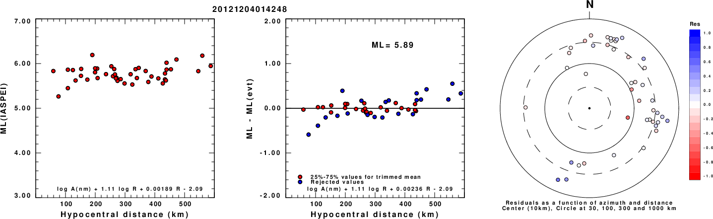
ML Magnitude
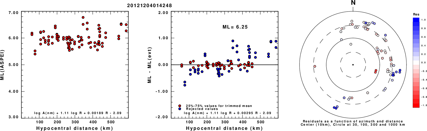
Left: ML computed using the IASPEI formula for Horizontal components. Center: ML residuals computed using a modified IASPEI formula that accounts for path specific attenuation; the values used for the trimmed mean are indicated. The ML relation used for each figure is given at the bottom of each plot.
Right: Residuals from new relation as a function of distance and azimuth.
Left: ML computed using the IASPEI formula for Vertical components (research). Center: ML residuals computed using a modified IASPEI formula that accounts for path specific attenuation; the values used for the trimmed mean are indicated. The ML relation used for each figure is given at the bottom of each plot.
Right: Residuals from new relation as a function of distance and azimuth.
Context
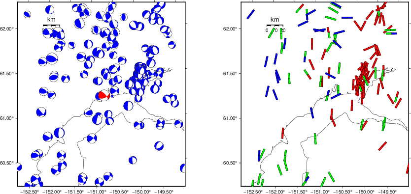
The left panel of the next figure presents the focal mechanism for this earthquake (red) in the context of other nearby events (blue) in the SLU Moment Tensor Catalog. The right panel shows the inferred direction of maximum compressive stress and the type of faulting (green is strike-slip, red is normal, blue is thrust; oblique is shown by a combination of colors). Thus context plot is useful for assessing the appropriateness of the moment tensor of this event.
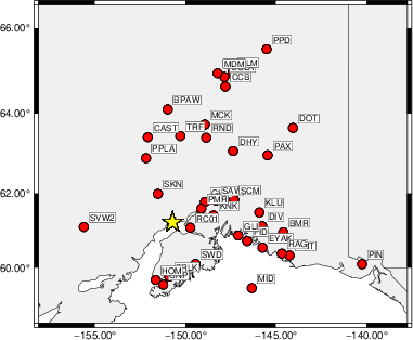
Waveform Inversion using wvfgrd96
The focal mechanism was determined using broadband seismic waveforms. The location of the event (star) and the
stations used for (red) the waveform inversion are shown in the next figure.
|
|
Location of broadband stations used for waveform inversion
|
The program wvfgrd96 was used with good traces observed at short distance to determine the focal mechanism, depth and seismic moment. This technique requires a high quality signal and well determined velocity model for the Green's functions. To the extent that these are the quality data, this type of mechanism should be preferred over the radiation pattern technique which requires the separate step of defining the pressure and tension quadrants and the correct strike.
The observed and predicted traces are filtered using the following gsac commands:
hp c 0.02 n 3
lp c 0.05 n 3
The results of this grid search are as follow:
           DEPTH  STK   DIP  RAKE   MW    FIT
WVFGRD96    1.0   210    50   -75   4.97 0.2202
WVFGRD96    2.0   220    60   -45   5.05 0.2827
WVFGRD96    3.0   205    50   -70   5.13 0.3112
WVFGRD96    4.0   225    80   -25   5.10 0.3220
WVFGRD96    5.0   230    90   -15   5.11 0.3377
WVFGRD96    6.0    50    85    15   5.14 0.3551
WVFGRD96    7.0    50    80    10   5.16 0.3721
WVFGRD96    8.0    50    75    10   5.19 0.3887
WVFGRD96    9.0    50    75    10   5.21 0.4020
WVFGRD96   10.0    50    75    10   5.22 0.4134
WVFGRD96   11.0    50    75    10   5.24 0.4229
WVFGRD96   12.0    50    75    10   5.25 0.4309
WVFGRD96   13.0    55    70    10   5.25 0.4391
WVFGRD96   14.0    55    70    10   5.26 0.4482
WVFGRD96   15.0    55    70    15   5.27 0.4598
WVFGRD96   16.0    55    70    15   5.28 0.4725
WVFGRD96   17.0    55    70    15   5.29 0.4851
WVFGRD96   18.0    55    70    15   5.30 0.4973
WVFGRD96   19.0    55    70    15   5.31 0.5091
WVFGRD96   20.0    55    70    15   5.32 0.5205
WVFGRD96   21.0    55    70    15   5.33 0.5310
WVFGRD96   22.0    55    70    15   5.34 0.5417
WVFGRD96   23.0    55    70    15   5.34 0.5520
WVFGRD96   24.0    55    70    15   5.35 0.5619
WVFGRD96   25.0    55    70    15   5.36 0.5714
WVFGRD96   26.0    55    70    10   5.37 0.5808
WVFGRD96   27.0    55    70    10   5.38 0.5898
WVFGRD96   28.0    55    70    10   5.39 0.5985
WVFGRD96   29.0    60    65    15   5.39 0.6074
WVFGRD96   30.0    60    65    15   5.40 0.6160
WVFGRD96   31.0    60    65    15   5.41 0.6245
WVFGRD96   32.0    60    65    15   5.42 0.6326
WVFGRD96   33.0    60    65    15   5.43 0.6404
WVFGRD96   34.0    60    65    15   5.44 0.6482
WVFGRD96   35.0    60    65    15   5.45 0.6557
WVFGRD96   36.0    60    65    15   5.46 0.6633
WVFGRD96   37.0    60    65    15   5.47 0.6707
WVFGRD96   38.0    60    65    15   5.48 0.6780
WVFGRD96   39.0    60    65    10   5.49 0.6847
WVFGRD96   40.0    60    55    15   5.56 0.6904
WVFGRD96   41.0    60    55    15   5.57 0.6976
WVFGRD96   42.0    60    55    15   5.57 0.7043
WVFGRD96   43.0    60    60    20   5.58 0.7109
WVFGRD96   44.0    60    60    20   5.59 0.7173
WVFGRD96   45.0    60    60    20   5.60 0.7233
WVFGRD96   46.0    60    60    20   5.61 0.7292
WVFGRD96   47.0    60    60    20   5.61 0.7348
WVFGRD96   48.0    60    60    20   5.62 0.7403
WVFGRD96   49.0    60    60    20   5.63 0.7455
WVFGRD96   50.0    65    55    20   5.63 0.7503
WVFGRD96   51.0    65    55    20   5.64 0.7550
WVFGRD96   52.0    65    55    25   5.64 0.7593
WVFGRD96   53.0    65    55    25   5.65 0.7631
WVFGRD96   54.0    65    55    25   5.65 0.7667
WVFGRD96   55.0    65    55    25   5.66 0.7698
WVFGRD96   56.0    65    55    25   5.67 0.7726
WVFGRD96   57.0    65    55    25   5.67 0.7750
WVFGRD96   58.0    65    55    25   5.68 0.7769
WVFGRD96   59.0    65    55    25   5.68 0.7784
WVFGRD96   60.0    65    55    25   5.69 0.7796
WVFGRD96   61.0    65    55    25   5.69 0.7804
WVFGRD96   62.0    65    55    25   5.69 0.7805
WVFGRD96   63.0    65    55    25   5.70 0.7805
WVFGRD96   64.0    65    55    25   5.70 0.7804
WVFGRD96   65.0    65    55    25   5.71 0.7793
WVFGRD96   66.0    65    55    25   5.71 0.7783
WVFGRD96   67.0    65    55    25   5.71 0.7771
WVFGRD96   68.0    65    55    25   5.72 0.7753
WVFGRD96   69.0    65    55    25   5.72 0.7734
WVFGRD96   70.0    65    55    25   5.72 0.7709
WVFGRD96   71.0    65    55    25   5.73 0.7683
WVFGRD96   72.0    65    55    25   5.73 0.7661
WVFGRD96   73.0    65    55    25   5.73 0.7632
WVFGRD96   74.0    65    55    25   5.73 0.7602
WVFGRD96   75.0    65    55    25   5.74 0.7574
WVFGRD96   76.0    65    55    25   5.74 0.7540
WVFGRD96   77.0    65    55    25   5.74 0.7507
WVFGRD96   78.0    65    55    25   5.74 0.7469
WVFGRD96   79.0    65    55    25   5.75 0.7432
WVFGRD96   80.0    65    55    25   5.75 0.7391
WVFGRD96   81.0    65    55    25   5.75 0.7352
WVFGRD96   82.0    65    55    25   5.75 0.7305
WVFGRD96   83.0    65    55    25   5.75 0.7264
WVFGRD96   84.0    65    55    25   5.76 0.7220
WVFGRD96   85.0    65    55    25   5.76 0.7172
WVFGRD96   86.0    65    55    25   5.76 0.7126
WVFGRD96   87.0    70    55    25   5.76 0.7081
WVFGRD96   88.0    70    55    25   5.76 0.7036
WVFGRD96   89.0    70    55    25   5.76 0.6988
WVFGRD96   90.0    70    55    25   5.76 0.6946
WVFGRD96   91.0    70    55    25   5.76 0.6900
WVFGRD96   92.0    70    55    25   5.76 0.6852
WVFGRD96   93.0    70    55    25   5.76 0.6806
WVFGRD96   94.0    70    55    25   5.76 0.6756
WVFGRD96   95.0    70    55    25   5.77 0.6712
WVFGRD96   96.0    70    55    25   5.77 0.6664
WVFGRD96   97.0    70    55    25   5.77 0.6617
WVFGRD96   98.0    70    55    25   5.77 0.6569
WVFGRD96   99.0    70    55    25   5.77 0.6527
WVFGRD96  100.0    70    55    25   5.77 0.6479
WVFGRD96  101.0    70    55    25   5.77 0.6437
WVFGRD96  102.0    70    55    25   5.77 0.6392
WVFGRD96  103.0    70    55    25   5.77 0.6349
WVFGRD96  104.0    70    55    25   5.78 0.6307
WVFGRD96  105.0    70    55    25   5.78 0.6261
WVFGRD96  106.0    70    55    20   5.78 0.6224
WVFGRD96  107.0    70    55    20   5.78 0.6182
WVFGRD96  108.0    70    55    20   5.78 0.6147
WVFGRD96  109.0    70    55    20   5.78 0.6107
WVFGRD96  110.0    70    55    20   5.78 0.6068
WVFGRD96  111.0    70    55    20   5.79 0.6031
WVFGRD96  112.0    70    55    20   5.79 0.5991
WVFGRD96  113.0    70    55    20   5.79 0.5957
WVFGRD96  114.0    70    55    20   5.79 0.5920
WVFGRD96  115.0    70    55    20   5.79 0.5884
WVFGRD96  116.0    65    60    20   5.79 0.5849
WVFGRD96  117.0    65    60    20   5.79 0.5813
WVFGRD96  118.0    65    60    20   5.79 0.5782
WVFGRD96  119.0    65    60    20   5.79 0.5747
WVFGRD96  120.0    65    60    20   5.80 0.5714
WVFGRD96  121.0    65    60    20   5.80 0.5682
WVFGRD96  122.0    65    60    20   5.80 0.5653
WVFGRD96  123.0    65    60    20   5.80 0.5621
WVFGRD96  124.0    65    60    20   5.80 0.5594
WVFGRD96  125.0    65    60    20   5.80 0.5565
WVFGRD96  126.0    65    60    20   5.80 0.5534
WVFGRD96  127.0    65    60    20   5.80 0.5509
WVFGRD96  128.0    65    60    20   5.80 0.5479
WVFGRD96  129.0    65    60    20   5.80 0.5449
The best solution is
WVFGRD96 63.0 65 55 25 5.70 0.7805
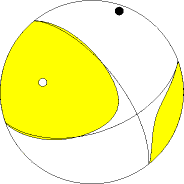
The mechanism corresponding to the best fit is
|
|
Figure 1. Waveform inversion focal mechanism
|
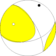
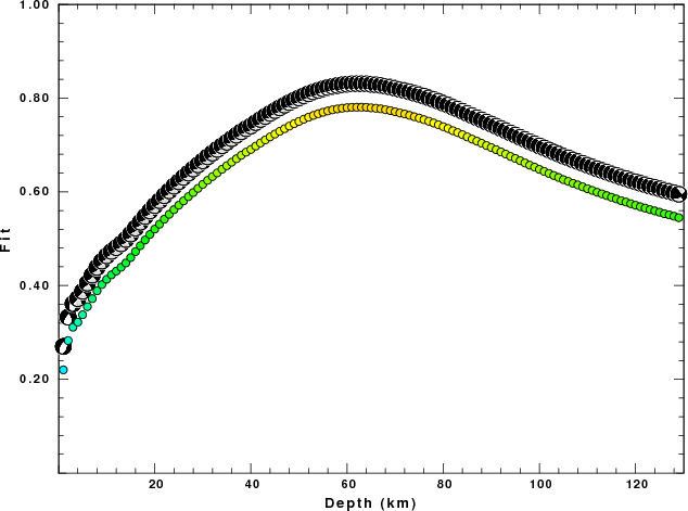
The best fit as a function of depth is given in the following figure:
|
|
Figure 2. Depth sensitivity for waveform mechanism
|
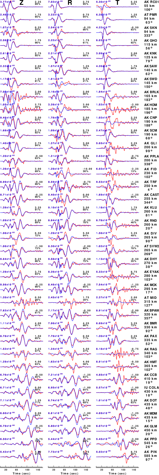
The comparison of the observed and predicted waveforms is given in the next figure. The red traces are the observed and the blue are the predicted.
Each observed-predicted component is plotted to the same scale and peak amplitudes are indicated by the numbers to the left of each trace. A pair of numbers is given in black at the right of each predicted traces. The upper number it the time shift required for maximum correlation between the observed and predicted traces. This time shift is required because the synthetics are not computed at exactly the same distance as the observed, the velocity model used in the predictions may not be perfect and the epicentral parameters may be be off.
A positive time shift indicates that the prediction is too fast and should be delayed to match the observed trace (shift to the right in this figure). A negative value indicates that the prediction is too slow. The lower number gives the percentage of variance reduction to characterize the individual goodness of fit (100% indicates a perfect fit).
The bandpass filter used in the processing and for the display was
hp c 0.02 n 3
lp c 0.05 n 3
|
|
Figure 3. Waveform comparison for selected depth. Red: observed; Blue - predicted. The time shift with respect to the model prediction is indicated. The percent of fit is also indicated. The time scale is relative to the first trace sample.
|
|
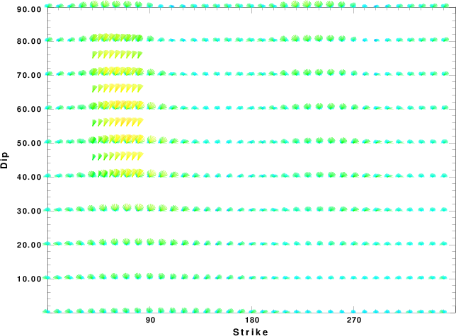
|
Focal mechanism sensitivity at the preferred depth. The red color indicates a very good fit to the waveforms.
Each solution is plotted as a vector at a given value of strike and dip with the angle of the vector representing the rake angle, measured, with respect to the upward vertical (N) in the figure.
|
A check on the assumed source location is possible by looking at the time shifts between the observed and predicted traces. The time shifts for waveform matching arise for several reasons:
- The origin time and epicentral distance are incorrect
- The velocity model used for the inversion is incorrect
- The velocity model used to define the P-arrival time is not the
same as the velocity model used for the waveform inversion
(assuming that the initial trace alignment is based on the
P arrival time)
Assuming only a mislocation, the time shifts are fit to a functional form:
Time_shift = A + B cos Azimuth + C Sin Azimuth
The time shifts for this inversion lead to the next figure:
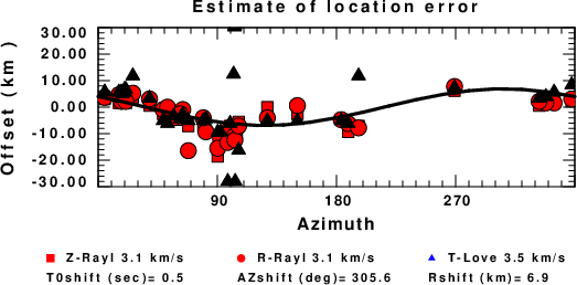
The derived shift in origin time and epicentral coordinates are given at the bottom of the figure.
Velocity Model
The WUS.model used for the waveform synthetic seismograms and for the surface wave eigenfunctions and dispersion is as follows
(The format is in the model96 format of Computer Programs in Seismology).
MODEL.01
Model after     8 iterations
ISOTROPIC
KGS
FLAT EARTH
1-D
CONSTANT VELOCITY
LINE08
LINE09
LINE10
LINE11
      H(KM)   VP(KM/S)   VS(KM/S) RHO(GM/CC)         QP         QS       ETAP       ETAS      FREFP      FREFS
     1.9000     3.4065     2.0089     2.2150  0.302E-02  0.679E-02   0.00       0.00       1.00       1.00
     6.1000     5.5445     3.2953     2.6089  0.349E-02  0.784E-02   0.00       0.00       1.00       1.00
    13.0000     6.2708     3.7396     2.7812  0.212E-02  0.476E-02   0.00       0.00       1.00       1.00
    19.0000     6.4075     3.7680     2.8223  0.111E-02  0.249E-02   0.00       0.00       1.00       1.00
     0.0000     7.9000     4.6200     3.2760  0.164E-10  0.370E-10   0.00       0.00       1.00       1.00
Last Changed Sat Apr 27 12:40:46 AM CDT 2024