Location
Location ANSS
The ANSS event ID is ak012fftc799 and the event page is at
https://earthquake.usgs.gov/earthquakes/eventpage/ak012fftc799/executive.
2012/12/01 08:00:57 58.423 -154.118 84.7 5.4 Alaska
Focal Mechanism
 USGS/SLU Moment Tensor Solution
 ENS  2012/12/01 08:00:57:0  58.42 -154.12  84.7 5.4 Alaska

 Stations used:
   AK.BRLK AK.CAST AK.CNP AK.EYAK AK.FID AK.HOM AK.KNK AK.PPLA
   AK.PWL AK.RC01 AK.SAW AK.SCM AK.SII AK.SWD AT.CHGN AT.MID
   AT.OHAK AT.PMR AT.SVW2

 Filtering commands used:
   hp c 0.02 n 3
   lp c 0.05 n 3

 Best Fitting Double Couple
  Mo = 1.24e+24 dyne-cm
  Mw = 5.33
  Z  = 92 km
  Plane   Strike  Dip  Rake
   NP1       65    85    55
   NP2      328    35   171
  Principal Axes:
   Axis    Value   Plunge  Azimuth
    T   1.24e+24     40     303
    N   0.00e+00     35      68
    P  -1.24e+24     31     183

 Moment Tensor: (dyne-cm)
    Component   Value
       Mxx    -6.90e+23
       Mxy    -3.89e+23
       Mxz     8.84e+23
       Myy     5.13e+23
       Myz    -4.81e+23
       Mzz     1.77e+23


                     --------------
                 ########--------------
              ################------------
             ####################----------
           ########################----------
          ###########################---------
         #######   ####################-------#
        ######## T #####################---#####
        ########   #####################-#######
       ##############################-----#######
       ##########################---------#######
       ######################--------------######
       ##################------------------######
        #############----------------------#####
        ########---------------------------#####
         ##--------------------------------####
          ---------------------------------###
           ---------------   -------------###
             ------------- P ------------##
              ------------   -----------##
                 ----------------------
                     --------------


 Global CMT Convention Moment Tensor:
      R          T          P
  1.77e+23   8.84e+23   4.81e+23
  8.84e+23  -6.90e+23   3.89e+23
  4.81e+23   3.89e+23   5.13e+23


Details of the solution is found at

http://www.eas.slu.edu/eqc/eqc_mt/MECH.NA/20121201080057/index.html
|
Preferred Solution
The preferred solution from an analysis of the surface-wave spectral amplitude radiation pattern, waveform inversion or first motion observations is
      STK = 65
      DIP = 85
     RAKE = 55
       MW = 5.33
       HS = 92.0
The NDK file is 20121201080057.ndk
The waveform inversion is preferred.
Moment Tensor Comparison
The following compares this source inversion to those provided by others. The purpose is to look for major differences and also to note slight differences that might be inherent to the processing procedure. For completeness the USGS/SLU solution is repeated from above.
| SLU |
USGSMT |
 USGS/SLU Moment Tensor Solution
 ENS  2012/12/01 08:00:57:0  58.42 -154.12  84.7 5.4 Alaska

 Stations used:
   AK.BRLK AK.CAST AK.CNP AK.EYAK AK.FID AK.HOM AK.KNK AK.PPLA
   AK.PWL AK.RC01 AK.SAW AK.SCM AK.SII AK.SWD AT.CHGN AT.MID
   AT.OHAK AT.PMR AT.SVW2

 Filtering commands used:
   hp c 0.02 n 3
   lp c 0.05 n 3

 Best Fitting Double Couple
  Mo = 1.24e+24 dyne-cm
  Mw = 5.33
  Z  = 92 km
  Plane   Strike  Dip  Rake
   NP1       65    85    55
   NP2      328    35   171
  Principal Axes:
   Axis    Value   Plunge  Azimuth
    T   1.24e+24     40     303
    N   0.00e+00     35      68
    P  -1.24e+24     31     183

 Moment Tensor: (dyne-cm)
    Component   Value
       Mxx    -6.90e+23
       Mxy    -3.89e+23
       Mxz     8.84e+23
       Myy     5.13e+23
       Myz    -4.81e+23
       Mzz     1.77e+23


                     --------------
                 ########--------------
              ################------------
             ####################----------
           ########################----------
          ###########################---------
         #######   ####################-------#
        ######## T #####################---#####
        ########   #####################-#######
       ##############################-----#######
       ##########################---------#######
       ######################--------------######
       ##################------------------######
        #############----------------------#####
        ########---------------------------#####
         ##--------------------------------####
          ---------------------------------###
           ---------------   -------------###
             ------------- P ------------##
              ------------   -----------##
                 ----------------------
                     --------------


 Global CMT Convention Moment Tensor:
      R          T          P
  1.77e+23   8.84e+23   4.81e+23
  8.84e+23  -6.90e+23   3.89e+23
  4.81e+23   3.89e+23   5.13e+23


Details of the solution is found at

http://www.eas.slu.edu/eqc/eqc_mt/MECH.NA/20121201080057/index.html
|
USGS WPhase Moment Solution
ALASKA PENINSULA

12/12/01  8:00:57

Epicenter:  58.533 -154.180
MW 5.3

USGS/WPHASE CENTROID MOMENT TENSOR
12/12/01 08:00:57.00
Centroid:   58.433 -153.796
Depth 100         No. of sta: 35
Moment Tensor;   Scale 10**16 Nm
  Mrr= 4.21       Mtt=-9.92
  Mpp= 5.70       Mrt= 6.42
  Mrp= 4.37       Mtp= 0.09
 Principal axes:
  T  Val= 10.38  Plg=45  Azm=288
  N     =  2.15      36       67
  P     =-12.53      22      174

Best Double Couple:Mo=1.2*10**17
 NP1:Strike=310 Dip=40 Slip= 158
 NP2:        57     76        52
|
Magnitudes
Given the availability of digital waveforms for determination of the moment tensor, this section documents the added processing leading to mLg, if appropriate to the region, and ML by application of the respective IASPEI formulae. As a research study, the linear distance term of the IASPEI formula
for ML is adjusted to remove a linear distance trend in residuals to give a regionally defined ML. The defined ML uses horizontal component recordings, but the same procedure is applied to the vertical components since there may be some interest in vertical component ground motions. Residual plots versus distance may indicate interesting features of ground motion scaling in some distance ranges. A residual plot of the regionalized magnitude is given as a function of distance and azimuth, since data sets may transcend different wave propagation provinces.
ML Magnitude
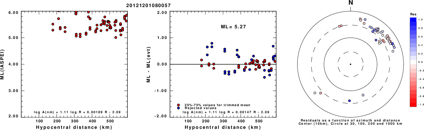
Left: ML computed using the IASPEI formula for Horizontal components. Center: ML residuals computed using a modified IASPEI formula that accounts for path specific attenuation; the values used for the trimmed mean are indicated. The ML relation used for each figure is given at the bottom of each plot.
Right: Residuals from new relation as a function of distance and azimuth.
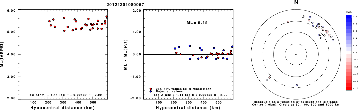
Left: ML computed using the IASPEI formula for Vertical components (research). Center: ML residuals computed using a modified IASPEI formula that accounts for path specific attenuation; the values used for the trimmed mean are indicated. The ML relation used for each figure is given at the bottom of each plot.
Right: Residuals from new relation as a function of distance and azimuth.
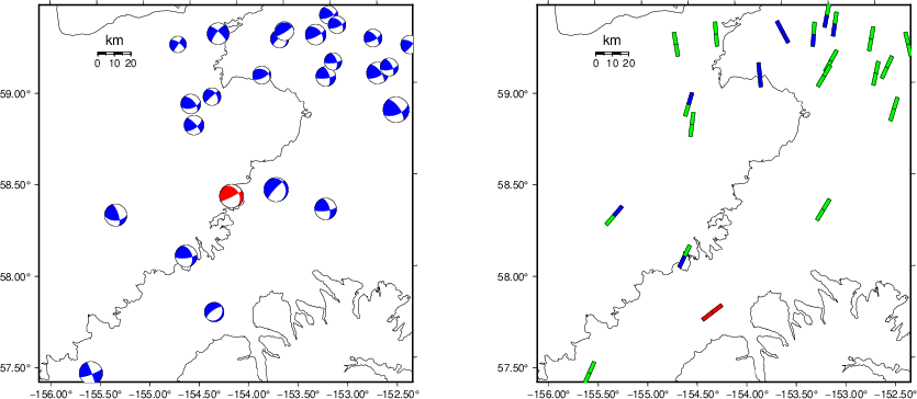
Context
The left panel of the next figure presents the focal mechanism for this earthquake (red) in the context of other nearby events (blue) in the SLU Moment Tensor Catalog. The right panel shows the inferred direction of maximum compressive stress and the type of faulting (green is strike-slip, red is normal, blue is thrust; oblique is shown by a combination of colors). Thus context plot is useful for assessing the appropriateness of the moment tensor of this event.
Waveform Inversion using wvfgrd96
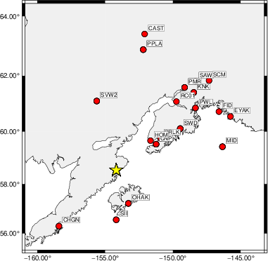
The focal mechanism was determined using broadband seismic waveforms. The location of the event (star) and the
stations used for (red) the waveform inversion are shown in the next figure.
|
|
Location of broadband stations used for waveform inversion
|
The program wvfgrd96 was used with good traces observed at short distance to determine the focal mechanism, depth and seismic moment. This technique requires a high quality signal and well determined velocity model for the Green's functions. To the extent that these are the quality data, this type of mechanism should be preferred over the radiation pattern technique which requires the separate step of defining the pressure and tension quadrants and the correct strike.
The observed and predicted traces are filtered using the following gsac commands:
hp c 0.02 n 3
lp c 0.05 n 3
The results of this grid search are as follow:
           DEPTH  STK   DIP  RAKE   MW    FIT
WVFGRD96    0.5    50    45   -65   4.50 0.1438
WVFGRD96    1.0    40    45   -80   4.54 0.1550
WVFGRD96    2.0    45    45   -75   4.61 0.1859
WVFGRD96    3.0    40    40   -85   4.67 0.2048
WVFGRD96    4.0   220    50   -90   4.71 0.2087
WVFGRD96    5.0   120    45   -60   4.64 0.2025
WVFGRD96    6.0   120    45   -55   4.66 0.2031
WVFGRD96    7.0   120    45   -55   4.67 0.1984
WVFGRD96    8.0   120    45   -55   4.70 0.2084
WVFGRD96    9.0   130    50   -45   4.68 0.1993
WVFGRD96   10.0   135    50   -30   4.67 0.1952
WVFGRD96   11.0   135    50   -25   4.67 0.1909
WVFGRD96   12.0   135    50   -25   4.67 0.1893
WVFGRD96   13.0   140    55   -20   4.67 0.1886
WVFGRD96   14.0   140    55   -15   4.67 0.1862
WVFGRD96   15.0   140    55   -15   4.68 0.1866
WVFGRD96   16.0   140    55   -15   4.68 0.1845
WVFGRD96   17.0   150    45    15   4.70 0.1876
WVFGRD96   18.0   150    45    15   4.71 0.1910
WVFGRD96   19.0   150    45    15   4.72 0.1916
WVFGRD96   20.0   150    45    15   4.73 0.1949
WVFGRD96   21.0    70    90    40   4.72 0.1963
WVFGRD96   22.0    70    90    40   4.74 0.2006
WVFGRD96   23.0    70    90    40   4.75 0.2048
WVFGRD96   24.0   250    85   -40   4.76 0.2100
WVFGRD96   25.0    70    90    40   4.77 0.2139
WVFGRD96   26.0    70    90    40   4.78 0.2185
WVFGRD96   27.0   250    85   -40   4.79 0.2250
WVFGRD96   28.0   245    80   -45   4.81 0.2303
WVFGRD96   29.0   245    80   -45   4.82 0.2359
WVFGRD96   30.0   245    80   -45   4.83 0.2416
WVFGRD96   31.0   245    80   -45   4.84 0.2471
WVFGRD96   32.0   245    80   -45   4.85 0.2526
WVFGRD96   33.0   245    80   -45   4.86 0.2581
WVFGRD96   34.0   250    80   -40   4.87 0.2640
WVFGRD96   35.0   250    80   -40   4.89 0.2699
WVFGRD96   36.0   250    80   -35   4.90 0.2755
WVFGRD96   37.0   250    85   -35   4.91 0.2816
WVFGRD96   38.0   250    85   -35   4.93 0.2875
WVFGRD96   39.0   250    85   -30   4.95 0.2935
WVFGRD96   40.0   245    70   -50   5.04 0.3109
WVFGRD96   41.0   245    70   -50   5.05 0.3168
WVFGRD96   42.0   240    70   -50   5.06 0.3230
WVFGRD96   43.0   240    70   -50   5.07 0.3292
WVFGRD96   44.0   240    70   -50   5.08 0.3352
WVFGRD96   45.0   240    70   -50   5.09 0.3412
WVFGRD96   46.0   240    70   -50   5.10 0.3472
WVFGRD96   47.0   240    70   -50   5.11 0.3530
WVFGRD96   48.0   240    70   -50   5.12 0.3587
WVFGRD96   49.0   240    75   -50   5.13 0.3646
WVFGRD96   50.0   240    75   -50   5.14 0.3710
WVFGRD96   51.0   240    75   -45   5.15 0.3786
WVFGRD96   52.0   240    75   -45   5.15 0.3858
WVFGRD96   53.0   245    80   -45   5.16 0.3931
WVFGRD96   54.0   245    80   -45   5.17 0.4002
WVFGRD96   55.0   245    80   -45   5.18 0.4071
WVFGRD96   56.0   245    80   -45   5.18 0.4138
WVFGRD96   57.0   245    80   -45   5.19 0.4204
WVFGRD96   58.0   245    80   -45   5.20 0.4266
WVFGRD96   59.0   245    85   -45   5.21 0.4332
WVFGRD96   60.0   245    85   -45   5.21 0.4396
WVFGRD96   61.0   245    85   -45   5.22 0.4456
WVFGRD96   62.0   245    85   -45   5.23 0.4513
WVFGRD96   63.0   245    85   -45   5.23 0.4566
WVFGRD96   64.0   245    85   -45   5.24 0.4617
WVFGRD96   65.0   245    85   -45   5.24 0.4664
WVFGRD96   66.0   245    85   -45   5.25 0.4707
WVFGRD96   67.0   245    85   -45   5.25 0.4748
WVFGRD96   68.0   245    85   -45   5.26 0.4787
WVFGRD96   69.0   245    85   -45   5.26 0.4823
WVFGRD96   70.0   245    85   -45   5.27 0.4855
WVFGRD96   71.0   245    85   -45   5.27 0.4884
WVFGRD96   72.0   245    85   -45   5.27 0.4918
WVFGRD96   73.0   240    85   -50   5.29 0.4952
WVFGRD96   74.0    65    90    50   5.28 0.4989
WVFGRD96   75.0   245    90   -50   5.29 0.5034
WVFGRD96   76.0    65    90    50   5.29 0.5075
WVFGRD96   77.0    65    90    50   5.29 0.5112
WVFGRD96   78.0    65    90    50   5.30 0.5144
WVFGRD96   79.0    65    90    50   5.30 0.5173
WVFGRD96   80.0    65    90    50   5.30 0.5200
WVFGRD96   81.0    65    90    50   5.31 0.5225
WVFGRD96   82.0   245    90   -50   5.31 0.5246
WVFGRD96   83.0    65    90    50   5.31 0.5260
WVFGRD96   84.0    65    90    50   5.31 0.5274
WVFGRD96   85.0   245    90   -50   5.31 0.5285
WVFGRD96   86.0    65    90    50   5.32 0.5291
WVFGRD96   87.0   245    90   -50   5.32 0.5296
WVFGRD96   88.0    65    90    55   5.32 0.5304
WVFGRD96   89.0   245    90   -55   5.33 0.5308
WVFGRD96   90.0   245    90   -55   5.33 0.5307
WVFGRD96   91.0    65    85    55   5.32 0.5312
WVFGRD96   92.0    65    85    55   5.33 0.5312
WVFGRD96   93.0   245    90   -55   5.33 0.5299
WVFGRD96   94.0    65    85    55   5.33 0.5301
WVFGRD96   95.0   245    90   -55   5.33 0.5278
WVFGRD96   96.0    65    85    55   5.33 0.5284
WVFGRD96   97.0    65    85    55   5.33 0.5270
WVFGRD96   98.0    65    85    55   5.33 0.5255
WVFGRD96   99.0    65    85    55   5.33 0.5240
WVFGRD96  100.0    65    85    55   5.33 0.5223
WVFGRD96  101.0    65    85    55   5.33 0.5203
WVFGRD96  102.0   245    90   -55   5.34 0.5148
WVFGRD96  103.0   245    90   -55   5.34 0.5125
WVFGRD96  104.0   240    90   -60   5.35 0.5103
WVFGRD96  105.0   240    90   -60   5.35 0.5075
WVFGRD96  106.0    65    85    60   5.34 0.5097
WVFGRD96  107.0    65    85    60   5.34 0.5073
WVFGRD96  108.0    65    85    60   5.34 0.5046
WVFGRD96  109.0    65    85    60   5.34 0.5020
WVFGRD96  110.0    65    85    60   5.34 0.4993
WVFGRD96  111.0    65    85    60   5.34 0.4963
WVFGRD96  112.0    65    85    60   5.34 0.4933
WVFGRD96  113.0    65    85    60   5.34 0.4904
WVFGRD96  114.0    65    85    60   5.34 0.4872
WVFGRD96  115.0    65    85    60   5.34 0.4841
WVFGRD96  116.0    65    85    60   5.34 0.4808
WVFGRD96  117.0    65    85    60   5.34 0.4775
WVFGRD96  118.0    65    85    60   5.34 0.4740
WVFGRD96  119.0    65    85    60   5.34 0.4707
WVFGRD96  120.0    65    85    60   5.34 0.4673
WVFGRD96  121.0    70    80    55   5.32 0.4638
WVFGRD96  122.0    70    80    55   5.32 0.4607
WVFGRD96  123.0    70    80    55   5.32 0.4573
WVFGRD96  124.0    70    80    55   5.32 0.4542
WVFGRD96  125.0    70    80    55   5.32 0.4508
WVFGRD96  126.0    70    80    55   5.32 0.4477
WVFGRD96  127.0    65    80    60   5.33 0.4443
WVFGRD96  128.0    65    80    60   5.33 0.4413
WVFGRD96  129.0    65    80    60   5.33 0.4380
The best solution is
WVFGRD96 92.0 65 85 55 5.33 0.5312
The mechanism corresponding to the best fit is
|
|
Figure 1. Waveform inversion focal mechanism
|
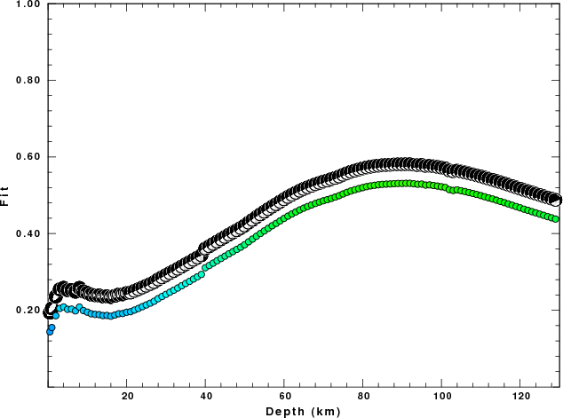
The best fit as a function of depth is given in the following figure:
|
|
Figure 2. Depth sensitivity for waveform mechanism
|
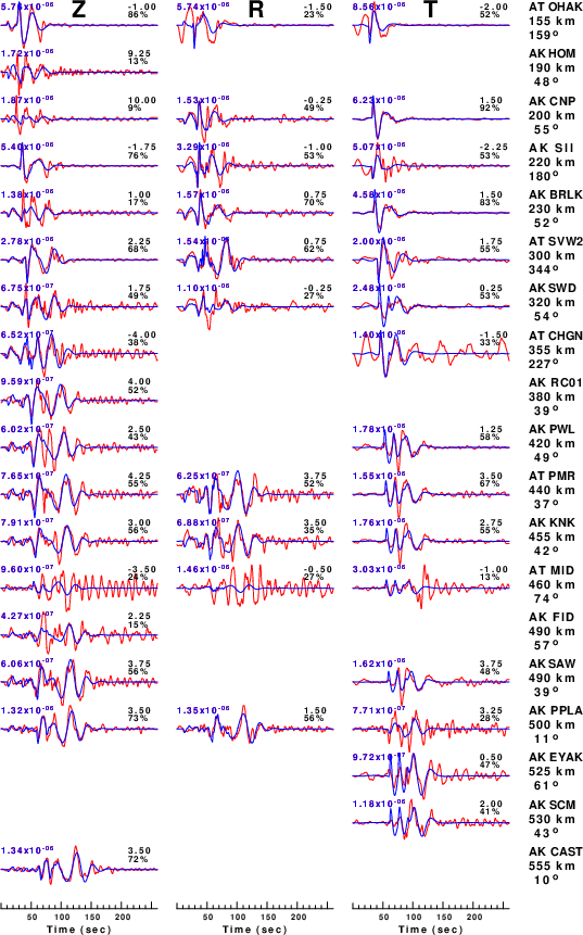
The comparison of the observed and predicted waveforms is given in the next figure. The red traces are the observed and the blue are the predicted.
Each observed-predicted component is plotted to the same scale and peak amplitudes are indicated by the numbers to the left of each trace. A pair of numbers is given in black at the right of each predicted traces. The upper number it the time shift required for maximum correlation between the observed and predicted traces. This time shift is required because the synthetics are not computed at exactly the same distance as the observed, the velocity model used in the predictions may not be perfect and the epicentral parameters may be be off.
A positive time shift indicates that the prediction is too fast and should be delayed to match the observed trace (shift to the right in this figure). A negative value indicates that the prediction is too slow. The lower number gives the percentage of variance reduction to characterize the individual goodness of fit (100% indicates a perfect fit).
The bandpass filter used in the processing and for the display was
hp c 0.02 n 3
lp c 0.05 n 3
|
|
Figure 3. Waveform comparison for selected depth. Red: observed; Blue - predicted. The time shift with respect to the model prediction is indicated. The percent of fit is also indicated. The time scale is relative to the first trace sample.
|
|
|
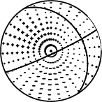
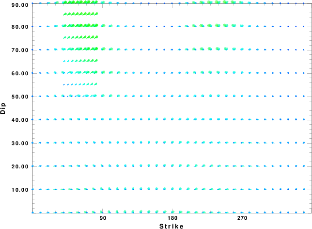
Focal mechanism sensitivity at the preferred depth. The red color indicates a very good fit to the waveforms.
Each solution is plotted as a vector at a given value of strike and dip with the angle of the vector representing the rake angle, measured, with respect to the upward vertical (N) in the figure.
|
A check on the assumed source location is possible by looking at the time shifts between the observed and predicted traces. The time shifts for waveform matching arise for several reasons:
- The origin time and epicentral distance are incorrect
- The velocity model used for the inversion is incorrect
- The velocity model used to define the P-arrival time is not the
same as the velocity model used for the waveform inversion
(assuming that the initial trace alignment is based on the
P arrival time)
Assuming only a mislocation, the time shifts are fit to a functional form:
Time_shift = A + B cos Azimuth + C Sin Azimuth
The time shifts for this inversion lead to the next figure:
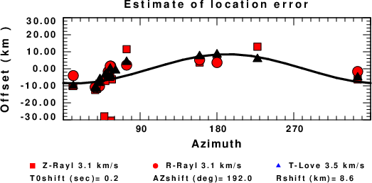
The derived shift in origin time and epicentral coordinates are given at the bottom of the figure.
Velocity Model
The WUS.model used for the waveform synthetic seismograms and for the surface wave eigenfunctions and dispersion is as follows
(The format is in the model96 format of Computer Programs in Seismology).
MODEL.01
Model after     8 iterations
ISOTROPIC
KGS
FLAT EARTH
1-D
CONSTANT VELOCITY
LINE08
LINE09
LINE10
LINE11
      H(KM)   VP(KM/S)   VS(KM/S) RHO(GM/CC)         QP         QS       ETAP       ETAS      FREFP      FREFS
     1.9000     3.4065     2.0089     2.2150  0.302E-02  0.679E-02   0.00       0.00       1.00       1.00
     6.1000     5.5445     3.2953     2.6089  0.349E-02  0.784E-02   0.00       0.00       1.00       1.00
    13.0000     6.2708     3.7396     2.7812  0.212E-02  0.476E-02   0.00       0.00       1.00       1.00
    19.0000     6.4075     3.7680     2.8223  0.111E-02  0.249E-02   0.00       0.00       1.00       1.00
     0.0000     7.9000     4.6200     3.2760  0.164E-10  0.370E-10   0.00       0.00       1.00       1.00
Last Changed Sat Apr 27 12:16:18 AM CDT 2024