Location
SLU Location
To check the ANSS location or to compare the observed P-wave first motions to the moment tensor solution, P- and S-wave first arrival times were manually read together with the P-wave first motions. The subsequent output of the program elocate is given in the file elocate.txt. The first motion plot is shown below.
Location ANSS
The ANSS event ID is se609737 and the event page is at
https://earthquake.usgs.gov/earthquakes/eventpage/se609737/executive.
2012/11/10 17:08:12 37.139 -83.054 17.0 4.2 Kentucky
Focal Mechanism
 USGS/SLU Moment Tensor Solution
 ENS  2012/11/10 17:08:12:0  37.14  -83.05  17.0 4.2 Kentucky

 Stations used:
   IU.SSPA IU.WCI IU.WVT NM.BLO NM.PLAL NM.SIUC NM.UTMT
   TA.149A TA.150A TA.151A TA.152A TA.153A TA.154A TA.155A
   TA.156A TA.251A TA.252A TA.254A TA.255A TA.256A TA.257A
   TA.KMSC TA.L46A TA.L47A TA.L48A TA.L49A TA.M46A TA.M47A
   TA.M48A TA.M50A TA.M51A TA.M54A TA.N47A TA.N48A TA.N49A
   TA.N50A TA.N51A TA.N54A TA.O45A TA.O47A TA.O48A TA.O49A
   TA.O50A TA.O51A TA.O52A TA.P43A TA.P44A TA.P45A TA.P46A
   TA.P47A TA.P48A TA.P49A TA.P51A TA.P52A TA.P53A TA.Q43A
   TA.Q44A TA.Q46A TA.Q47A TA.Q48A TA.Q49A TA.Q50A TA.Q51A
   TA.Q52A TA.R44A TA.R45A TA.R46A TA.R47A TA.R48A TA.R49A
   TA.R50A TA.R52A TA.R58B TA.S45A TA.S46A TA.S47A TA.S48A
   TA.S49A TA.S51A TA.S52A TA.SFIN TA.T46A TA.T47A TA.T48A
   TA.T50A TA.T51A TA.U46A TA.U47A TA.U48A TA.U50A TA.U51A
   TA.U52A TA.U53A TA.V46A TA.V47A TA.V48A TA.V50A TA.V51A
   TA.V52A TA.V53A TA.W45A TA.W46A TA.W47A TA.W48A TA.W49A
   TA.W50A TA.W51A TA.W52A TA.W53A TA.X46A TA.X48A TA.X49A
   TA.X51A TA.X52A TA.X53A TA.Y48A TA.Y49A TA.Y50A TA.Y51A
   TA.Y52A TA.Y53A TA.Y54A TA.Z48A TA.Z49A TA.Z50A TA.Z51A
   TA.Z52A TA.Z53A TA.Z54A TA.Z55A US.AAM US.ACSO US.BLA
   US.CBN US.GOGA US.LRAL US.MCWV US.NHSC US.TZTN

 Filtering commands used:
   hp c 0.02 n 3
   lp c 0.10 n 3

 Best Fitting Double Couple
  Mo = 2.19e+22 dyne-cm
  Mw = 4.16
  Z  = 14 km
  Plane   Strike  Dip  Rake
   NP1      110    85   -30
   NP2      203    60   -174
  Principal Axes:
   Axis    Value   Plunge  Azimuth
    T   2.19e+22     17     160
    N   0.00e+00     60     281
    P  -2.19e+22     24      62

 Moment Tensor: (dyne-cm)
    Component   Value
       Mxx     1.38e+22
       Mxy    -1.38e+22
       Mxz    -9.56e+21
       Myy    -1.19e+22
       Myz    -5.24e+21
       Mzz    -1.90e+21


                     ##############
                 ################------
              ################------------
             ###############---------------
           ###############-------------------
          ###############---------------------
         ###############-----------------   ---
        --#############------------------ P ----
        -----#########-------------------   ----
       ----------####----------------------------
       -------------##---------------------------
       -------------#######----------------------
       ------------#############-----------------
        -----------###################----------
        ----------###########################---
         ---------#############################
          --------############################
           -------###########################
             -----##############   ########
              -----############# T #######
                 --#############   ####
                     ##############


 Global CMT Convention Moment Tensor:
      R          T          P
 -1.90e+21  -9.56e+21   5.24e+21
 -9.56e+21   1.38e+22   1.38e+22
  5.24e+21   1.38e+22  -1.19e+22


Details of the solution is found at

http://www.eas.slu.edu/eqc/eqc_mt/MECH.NA/20121110170812/index.html
|
Preferred Solution
The preferred solution from an analysis of the surface-wave spectral amplitude radiation pattern, waveform inversion or first motion observations is
      STK = 110
      DIP = 85
     RAKE = -30
       MW = 4.16
       HS = 14.0
The NDK file is 20121110170812.ndk
The waveform inversion is preferred.
Moment Tensor Comparison
The following compares this source inversion to those provided by others. The purpose is to look for major differences and also to note slight differences that might be inherent to the processing procedure. For completeness the USGS/SLU solution is repeated from above.
| SLU |
USGSMT |
SLUFM |
 USGS/SLU Moment Tensor Solution
 ENS  2012/11/10 17:08:12:0  37.14  -83.05  17.0 4.2 Kentucky

 Stations used:
   IU.SSPA IU.WCI IU.WVT NM.BLO NM.PLAL NM.SIUC NM.UTMT
   TA.149A TA.150A TA.151A TA.152A TA.153A TA.154A TA.155A
   TA.156A TA.251A TA.252A TA.254A TA.255A TA.256A TA.257A
   TA.KMSC TA.L46A TA.L47A TA.L48A TA.L49A TA.M46A TA.M47A
   TA.M48A TA.M50A TA.M51A TA.M54A TA.N47A TA.N48A TA.N49A
   TA.N50A TA.N51A TA.N54A TA.O45A TA.O47A TA.O48A TA.O49A
   TA.O50A TA.O51A TA.O52A TA.P43A TA.P44A TA.P45A TA.P46A
   TA.P47A TA.P48A TA.P49A TA.P51A TA.P52A TA.P53A TA.Q43A
   TA.Q44A TA.Q46A TA.Q47A TA.Q48A TA.Q49A TA.Q50A TA.Q51A
   TA.Q52A TA.R44A TA.R45A TA.R46A TA.R47A TA.R48A TA.R49A
   TA.R50A TA.R52A TA.R58B TA.S45A TA.S46A TA.S47A TA.S48A
   TA.S49A TA.S51A TA.S52A TA.SFIN TA.T46A TA.T47A TA.T48A
   TA.T50A TA.T51A TA.U46A TA.U47A TA.U48A TA.U50A TA.U51A
   TA.U52A TA.U53A TA.V46A TA.V47A TA.V48A TA.V50A TA.V51A
   TA.V52A TA.V53A TA.W45A TA.W46A TA.W47A TA.W48A TA.W49A
   TA.W50A TA.W51A TA.W52A TA.W53A TA.X46A TA.X48A TA.X49A
   TA.X51A TA.X52A TA.X53A TA.Y48A TA.Y49A TA.Y50A TA.Y51A
   TA.Y52A TA.Y53A TA.Y54A TA.Z48A TA.Z49A TA.Z50A TA.Z51A
   TA.Z52A TA.Z53A TA.Z54A TA.Z55A US.AAM US.ACSO US.BLA
   US.CBN US.GOGA US.LRAL US.MCWV US.NHSC US.TZTN

 Filtering commands used:
   hp c 0.02 n 3
   lp c 0.10 n 3

 Best Fitting Double Couple
  Mo = 2.19e+22 dyne-cm
  Mw = 4.16
  Z  = 14 km
  Plane   Strike  Dip  Rake
   NP1      110    85   -30
   NP2      203    60   -174
  Principal Axes:
   Axis    Value   Plunge  Azimuth
    T   2.19e+22     17     160
    N   0.00e+00     60     281
    P  -2.19e+22     24      62

 Moment Tensor: (dyne-cm)
    Component   Value
       Mxx     1.38e+22
       Mxy    -1.38e+22
       Mxz    -9.56e+21
       Myy    -1.19e+22
       Myz    -5.24e+21
       Mzz    -1.90e+21


                     ##############
                 ################------
              ################------------
             ###############---------------
           ###############-------------------
          ###############---------------------
         ###############-----------------   ---
        --#############------------------ P ----
        -----#########-------------------   ----
       ----------####----------------------------
       -------------##---------------------------
       -------------#######----------------------
       ------------#############-----------------
        -----------###################----------
        ----------###########################---
         ---------#############################
          --------############################
           -------###########################
             -----##############   ########
              -----############# T #######
                 --#############   ####
                     ##############


 Global CMT Convention Moment Tensor:
      R          T          P
 -1.90e+21  -9.56e+21   5.24e+21
 -9.56e+21   1.38e+22   1.38e+22
  5.24e+21   1.38e+22  -1.19e+22


Details of the solution is found at

http://www.eas.slu.edu/eqc/eqc_mt/MECH.NA/20121110170812/index.html
|
USGS/SLU Regional Moment Solution
EASTERN KENTUCKY

12/11/10 17:08:13.01

Epicenter:  37.110  -82.969
MW 4.2

USGS/SLU REGIONAL MOMENT TENSOR
Depth  16         No. of sta:105
Moment Tensor;   Scale 10**15 Nm
  Mrr=-0.67       Mtt= 1.89
  Mpp=-1.22       Mrt=-0.85
  Mrp= 0.87       Mtp= 1.44
 Principal axes:
  T  Val=  2.53  Plg= 9  Azm=161
  N       -0.04      56      265
  P       -2.49      32       65

Best Double Couple:Mo=2.5*10**15
 NP1:Strike=109 Dip=75 Slip= -30
 NP2:       208     61      -162
|
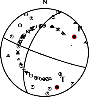
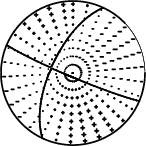
First motions and takeoff angles from an elocate run.
|
Magnitudes
Given the availability of digital waveforms for determination of the moment tensor, this section documents the added processing leading to mLg, if appropriate to the region, and ML by application of the respective IASPEI formulae. As a research study, the linear distance term of the IASPEI formula
for ML is adjusted to remove a linear distance trend in residuals to give a regionally defined ML. The defined ML uses horizontal component recordings, but the same procedure is applied to the vertical components since there may be some interest in vertical component ground motions. Residual plots versus distance may indicate interesting features of ground motion scaling in some distance ranges. A residual plot of the regionalized magnitude is given as a function of distance and azimuth, since data sets may transcend different wave propagation provinces.
mLg Magnitude
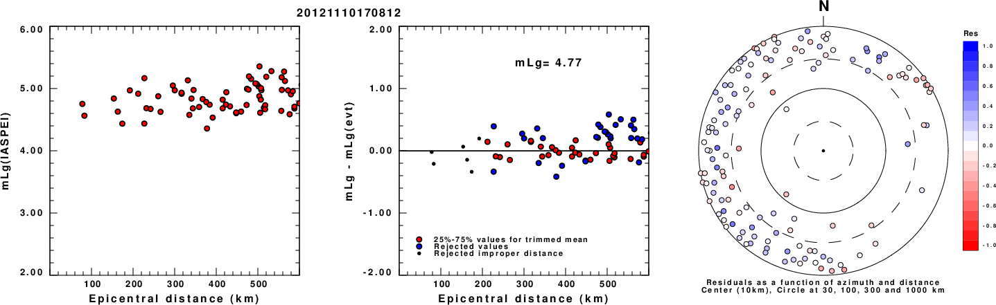
Left: mLg computed using the IASPEI formula. Center: mLg residuals versus epicentral distance ; the values used for the trimmed mean magnitude estimate are indicated.
Right: residuals as a function of distance and azimuth.
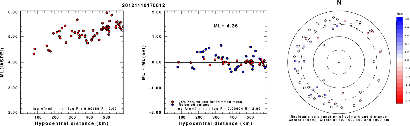
ML Magnitude
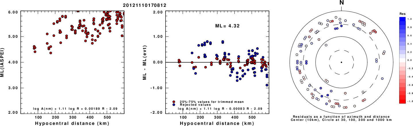
Left: ML computed using the IASPEI formula for Horizontal components. Center: ML residuals computed using a modified IASPEI formula that accounts for path specific attenuation; the values used for the trimmed mean are indicated. The ML relation used for each figure is given at the bottom of each plot.
Right: Residuals from new relation as a function of distance and azimuth.
Left: ML computed using the IASPEI formula for Vertical components (research). Center: ML residuals computed using a modified IASPEI formula that accounts for path specific attenuation; the values used for the trimmed mean are indicated. The ML relation used for each figure is given at the bottom of each plot.
Right: Residuals from new relation as a function of distance and azimuth.
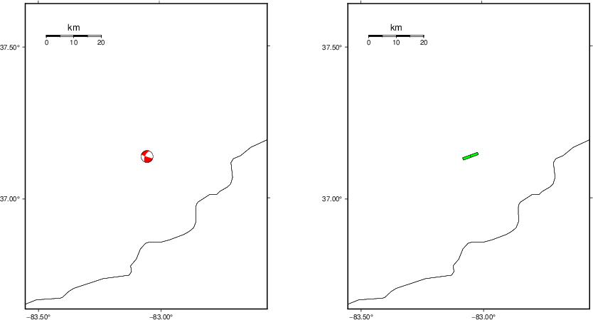
Context
The left panel of the next figure presents the focal mechanism for this earthquake (red) in the context of other nearby events (blue) in the SLU Moment Tensor Catalog. The right panel shows the inferred direction of maximum compressive stress and the type of faulting (green is strike-slip, red is normal, blue is thrust; oblique is shown by a combination of colors). Thus context plot is useful for assessing the appropriateness of the moment tensor of this event.
Waveform Inversion using wvfgrd96
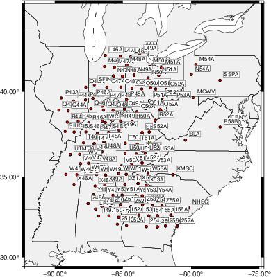
The focal mechanism was determined using broadband seismic waveforms. The location of the event (star) and the
stations used for (red) the waveform inversion are shown in the next figure.
|
|
Location of broadband stations used for waveform inversion
|
The program wvfgrd96 was used with good traces observed at short distance to determine the focal mechanism, depth and seismic moment. This technique requires a high quality signal and well determined velocity model for the Green's functions. To the extent that these are the quality data, this type of mechanism should be preferred over the radiation pattern technique which requires the separate step of defining the pressure and tension quadrants and the correct strike.
The observed and predicted traces are filtered using the following gsac commands:
hp c 0.02 n 3
lp c 0.10 n 3
The results of this grid search are as follow:
           DEPTH  STK   DIP  RAKE   MW    FIT
WVFGRD96    0.5   295    90     0   3.92 0.4666
WVFGRD96    1.0   295    90   -20   3.96 0.4858
WVFGRD96    2.0   290    80   -25   4.00 0.5067
WVFGRD96    3.0   295    80    30   4.03 0.5216
WVFGRD96    4.0   110    90   -35   4.03 0.5381
WVFGRD96    5.0   110    90   -35   4.04 0.5615
WVFGRD96    6.0   110    90   -30   4.05 0.5863
WVFGRD96    7.0   110    90   -30   4.06 0.6094
WVFGRD96    8.0   110    85   -30   4.08 0.6305
WVFGRD96    9.0   110    85   -30   4.09 0.6486
WVFGRD96   10.0   290    90    30   4.11 0.6619
WVFGRD96   11.0   110    85   -30   4.13 0.6764
WVFGRD96   12.0   110    85   -30   4.14 0.6853
WVFGRD96   13.0   110    85   -30   4.15 0.6909
WVFGRD96   14.0   110    85   -30   4.16 0.6933
WVFGRD96   15.0   110    85   -30   4.17 0.6928
WVFGRD96   16.0   110    85   -30   4.18 0.6896
WVFGRD96   17.0   110    85   -30   4.19 0.6841
WVFGRD96   18.0   110    85   -30   4.20 0.6768
WVFGRD96   19.0   110    85   -30   4.20 0.6678
WVFGRD96   20.0   110    85   -35   4.22 0.6564
WVFGRD96   21.0   110    85   -35   4.23 0.6450
WVFGRD96   22.0   110    85   -35   4.23 0.6327
WVFGRD96   23.0   110    85   -35   4.24 0.6191
WVFGRD96   24.0   110    85   -35   4.24 0.6048
WVFGRD96   25.0   110    90   -35   4.25 0.5908
WVFGRD96   26.0   290    90    35   4.25 0.5769
WVFGRD96   27.0   110    90   -35   4.26 0.5630
WVFGRD96   28.0   110    90   -35   4.26 0.5493
WVFGRD96   29.0   110    90   -35   4.27 0.5364
The best solution is
WVFGRD96 14.0 110 85 -30 4.16 0.6933
The mechanism corresponding to the best fit is
|
|
Figure 1. Waveform inversion focal mechanism
|
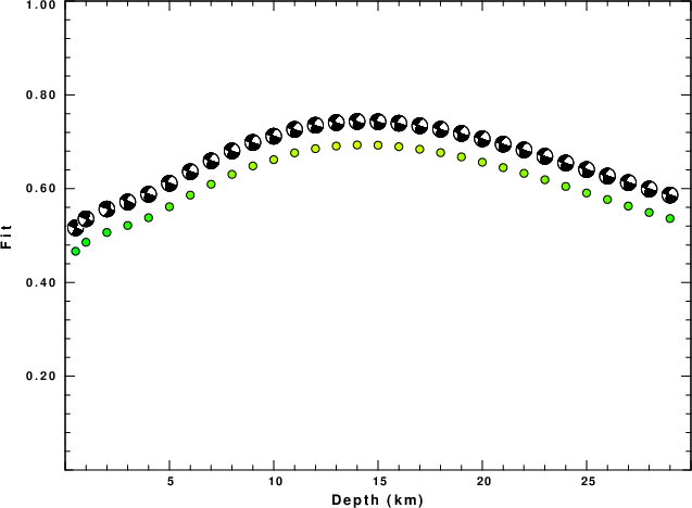
The best fit as a function of depth is given in the following figure:
|
|
Figure 2. Depth sensitivity for waveform mechanism
|
The comparison of the observed and predicted waveforms is given in the next figure. The red traces are the observed and the blue are the predicted.
Each observed-predicted component is plotted to the same scale and peak amplitudes are indicated by the numbers to the left of each trace. A pair of numbers is given in black at the right of each predicted traces. The upper number it the time shift required for maximum correlation between the observed and predicted traces. This time shift is required because the synthetics are not computed at exactly the same distance as the observed, the velocity model used in the predictions may not be perfect and the epicentral parameters may be be off.
A positive time shift indicates that the prediction is too fast and should be delayed to match the observed trace (shift to the right in this figure). A negative value indicates that the prediction is too slow. The lower number gives the percentage of variance reduction to characterize the individual goodness of fit (100% indicates a perfect fit).
The bandpass filter used in the processing and for the display was
hp c 0.02 n 3
lp c 0.10 n 3

|
|
Figure 3. Waveform comparison for selected depth. Red: observed; Blue - predicted. The time shift with respect to the model prediction is indicated. The percent of fit is also indicated. The time scale is relative to the first trace sample.
|
|
|
Focal mechanism sensitivity at the preferred depth. The red color indicates a very good fit to the waveforms.
Each solution is plotted as a vector at a given value of strike and dip with the angle of the vector representing the rake angle, measured, with respect to the upward vertical (N) in the figure.
|
A check on the assumed source location is possible by looking at the time shifts between the observed and predicted traces. The time shifts for waveform matching arise for several reasons:
- The origin time and epicentral distance are incorrect
- The velocity model used for the inversion is incorrect
- The velocity model used to define the P-arrival time is not the
same as the velocity model used for the waveform inversion
(assuming that the initial trace alignment is based on the
P arrival time)
Assuming only a mislocation, the time shifts are fit to a functional form:
Time_shift = A + B cos Azimuth + C Sin Azimuth
The time shifts for this inversion lead to the next figure:
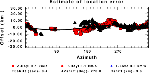
The derived shift in origin time and epicentral coordinates are given at the bottom of the figure.
Surface-Wave Focal Mechanism
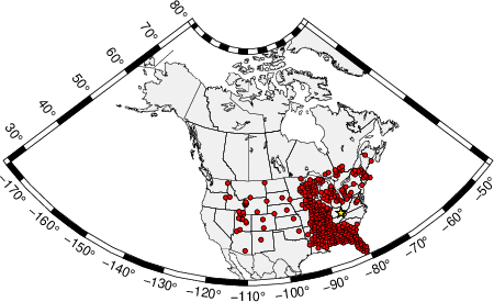
The following figure shows the stations used in the grid search for the best focal mechanism to fit the surface-wave spectral amplitudes of the Love and Rayleigh waves.
|
|
Location of broadband stations used to obtain focal mechanism from surface-wave spectral amplitudes
|
The surface-wave determined focal mechanism is shown here.
  NODAL PLANES


  STK=     112.87
  DIP=      85.46
 RAKE=     -25.08

             OR

  STK=     204.99
  DIP=      65.00
 RAKE=    -174.99


DEPTH = 14.0 km

Mw = 4.28
Best Fit 0.8225 - P-T axis plot gives solutions with FIT greater than FIT90
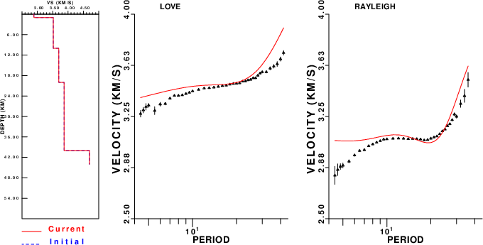
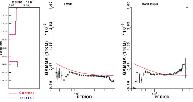
Surface-wave analysis
Surface wave analysis was performed using codes from
Computer Programs in Seismology, specifically the
multiple filter analysis program do_mft and the surface-wave
radiation pattern search program srfgrd96.
Data preparation
Digital data were collected, instrument response removed and traces converted
to Z, R an T components. Multiple filter analysis was applied to the Z and T traces to obtain the Rayleigh- and Love-wave spectral amplitudes, respectively.
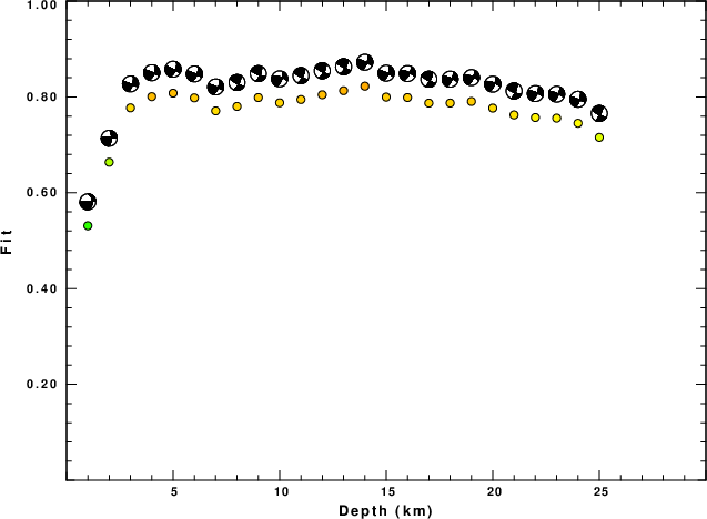
These were input to the search program which examined all depths between 1 and 25 km
and all possible mechanisms.
|
|
Best mechanism fit as a function of depth. The preferred depth is given above. Lower hemisphere projection
|
|
|
Pressure-tension axis trends. Since the surface-wave spectra search does not distinguish between P and T axes and since there is a 180 ambiguity in strike, all possible P and T axes are plotted. First motion data and waveforms will be used to select the preferred mechanism. The purpose of this plot is to provide an idea of the
possible range of solutions. The P and T-axes for all mechanisms with goodness of fit greater than 0.9 FITMAX (above) are plotted here.
|
|
|
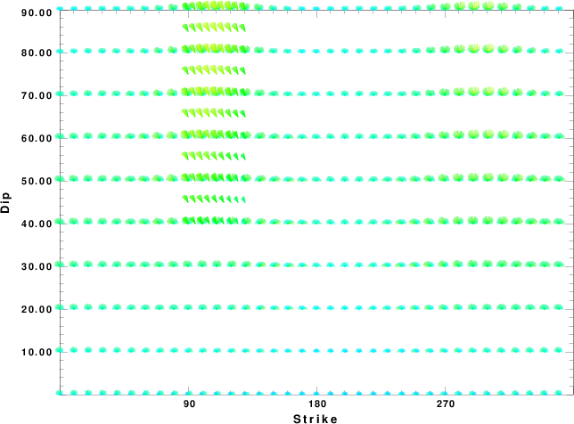
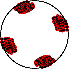
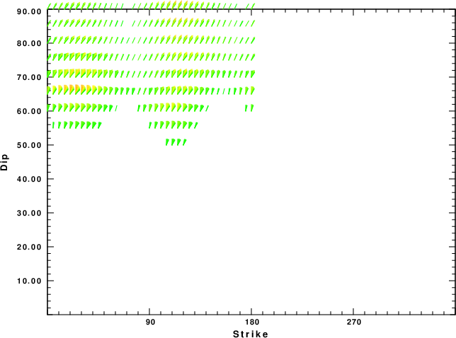
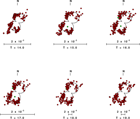
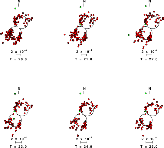
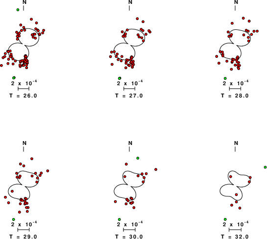
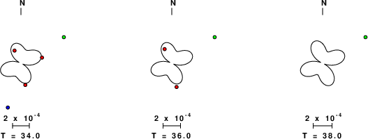
Focal mechanism sensitivity at the preferred depth. The red color indicates a very good fit to the Love and Rayleigh wave radiation patterns.
Each solution is plotted as a vector at a given value of strike and dip with the angle of the vector representing the rake angle, measured, with respect to the upward vertical (N) in the figure. Because of the symmetry of the spectral amplitude rediation patterns, only strikes from 0-180 degrees are sampled.
|
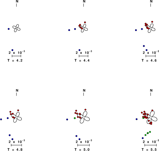
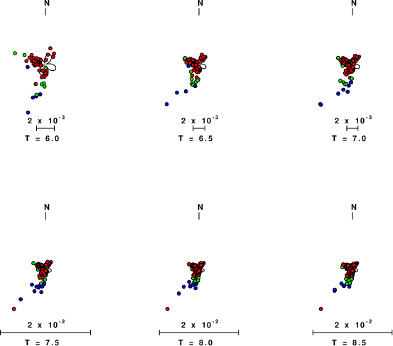
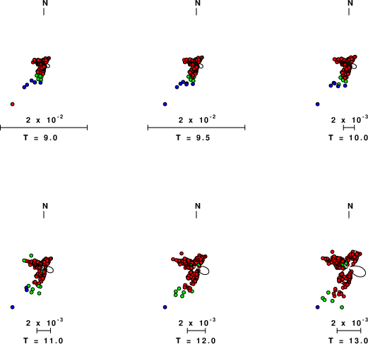
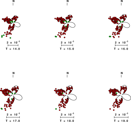
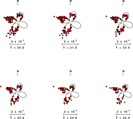
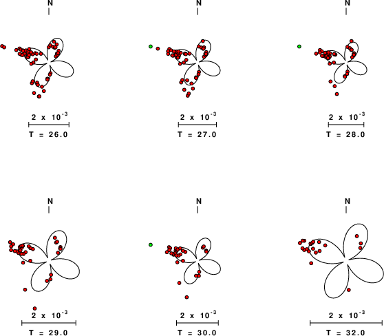
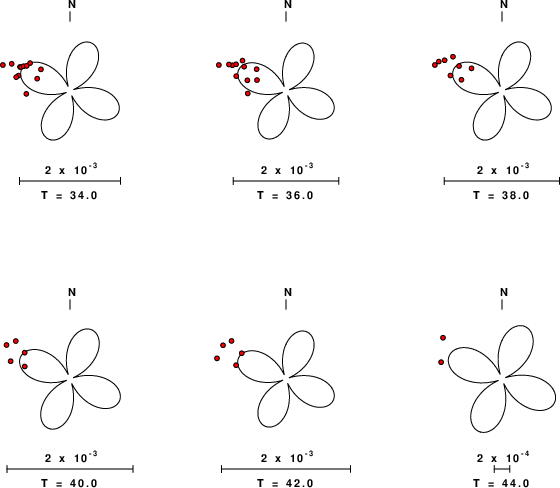
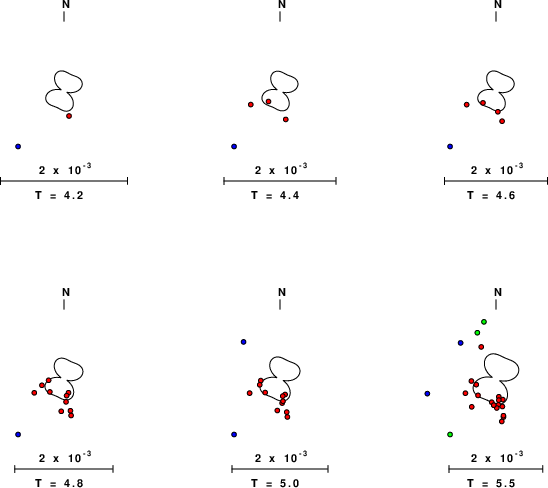
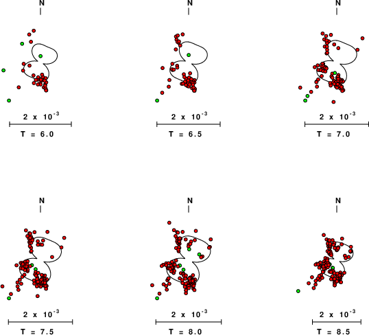
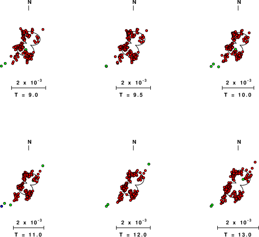
Love-wave radiation patterns
Rayleigh-wave radiation patterns