Location
Location ANSS
The ANSS event ID is ak012dz4hkhx and the event page is at
https://earthquake.usgs.gov/earthquakes/eventpage/ak012dz4hkhx/executive.
2012/10/30 22:02:46 61.493 -150.722 65.0 4.3 Alaska
Focal Mechanism
 USGS/SLU Moment Tensor Solution
 ENS  2012/10/30 22:02:46:0  61.49 -150.72  65.0 4.3 Alaska

 Stations used:
   AK.BPAW AK.BRLK AK.CAST AK.CNP AK.EYAK AK.FIB AK.FID AK.GHO
   AK.GLI AK.HIN AK.KLU AK.KNK AK.MCK AK.PPLA AK.PWL AK.RC01
   AK.RND AK.SAW AK.SCM AK.SKN AK.SWD AK.TRF AT.SVW2

 Filtering commands used:
   hp c 0.02 n 3
   lp c 0.06 n 3

 Best Fitting Double Couple
  Mo = 5.37e+22 dyne-cm
  Mw = 4.42
  Z  = 66 km
  Plane   Strike  Dip  Rake
   NP1      195    65   -70
   NP2      334    32   -126
  Principal Axes:
   Axis    Value   Plunge  Azimuth
    T   5.37e+22     18     270
    N   0.00e+00     18       6
    P  -5.37e+22     64     139

 Moment Tensor: (dyne-cm)
    Component   Value
       Mxx    -5.73e+21
       Mxy     4.75e+21
       Mxz     1.59e+22
       Myy     4.44e+22
       Myz    -2.93e+22
       Mzz    -3.87e+22


                     -----------###
                 ############-#########
              ###############----#########
             ##############--------########
           ###############-----------########
          ###############-------------########
         ###############----------------#######
        ###############------------------#######
        ###############-------------------######
       ##   ##########--------------------#######
       ## T ##########---------------------######
       ##   #########----------------------######
       ##############----------   ---------######
        #############---------- P ---------#####
        ############-----------   ---------#####
         ###########-----------------------####
          ##########----------------------####
           #########----------------------###
             ########--------------------##
              #######-------------------##
                 #####----------------#
                     #-------------


 Global CMT Convention Moment Tensor:
      R          T          P
 -3.87e+22   1.59e+22   2.93e+22
  1.59e+22  -5.73e+21  -4.75e+21
  2.93e+22  -4.75e+21   4.44e+22


Details of the solution is found at

http://www.eas.slu.edu/eqc/eqc_mt/MECH.NA/20121030220246/index.html
|
Preferred Solution
The preferred solution from an analysis of the surface-wave spectral amplitude radiation pattern, waveform inversion or first motion observations is
      STK = 195
      DIP = 65
     RAKE = -70
       MW = 4.42
       HS = 66.0
The NDK file is 20121030220246.ndk
The waveform inversion is preferred.
Magnitudes
Given the availability of digital waveforms for determination of the moment tensor, this section documents the added processing leading to mLg, if appropriate to the region, and ML by application of the respective IASPEI formulae. As a research study, the linear distance term of the IASPEI formula
for ML is adjusted to remove a linear distance trend in residuals to give a regionally defined ML. The defined ML uses horizontal component recordings, but the same procedure is applied to the vertical components since there may be some interest in vertical component ground motions. Residual plots versus distance may indicate interesting features of ground motion scaling in some distance ranges. A residual plot of the regionalized magnitude is given as a function of distance and azimuth, since data sets may transcend different wave propagation provinces.
ML Magnitude
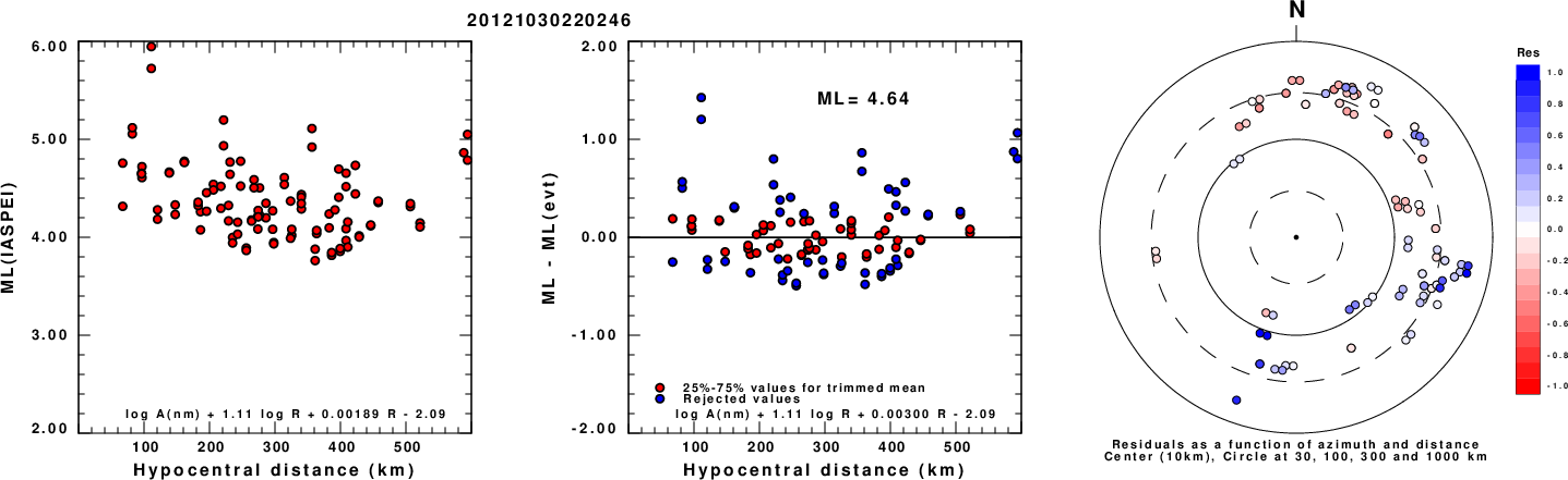
Left: ML computed using the IASPEI formula for Horizontal components. Center: ML residuals computed using a modified IASPEI formula that accounts for path specific attenuation; the values used for the trimmed mean are indicated. The ML relation used for each figure is given at the bottom of each plot.
Right: Residuals from new relation as a function of distance and azimuth.
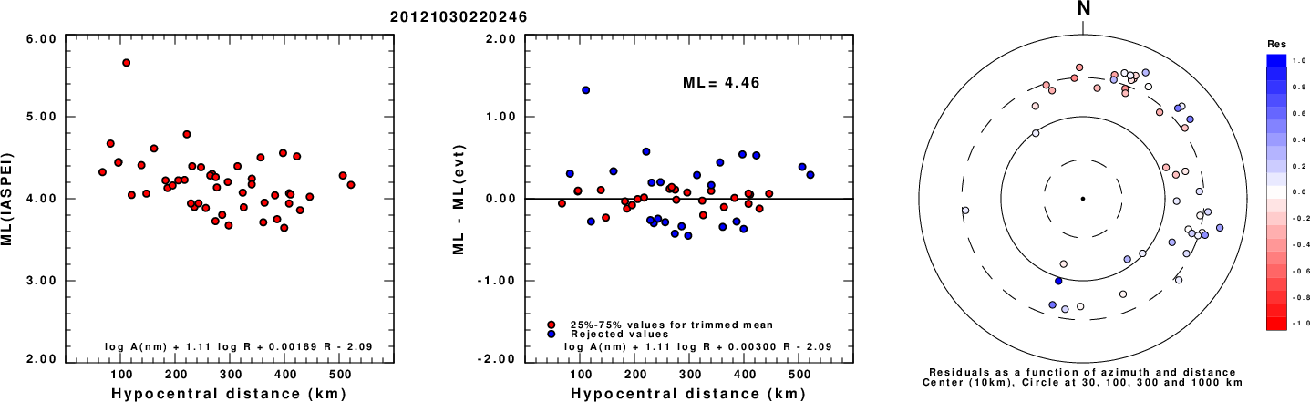
Left: ML computed using the IASPEI formula for Vertical components (research). Center: ML residuals computed using a modified IASPEI formula that accounts for path specific attenuation; the values used for the trimmed mean are indicated. The ML relation used for each figure is given at the bottom of each plot.
Right: Residuals from new relation as a function of distance and azimuth.
Context
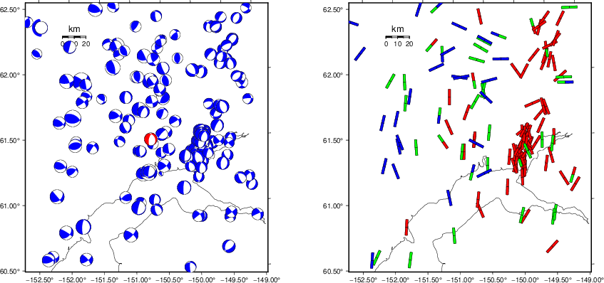
The left panel of the next figure presents the focal mechanism for this earthquake (red) in the context of other nearby events (blue) in the SLU Moment Tensor Catalog. The right panel shows the inferred direction of maximum compressive stress and the type of faulting (green is strike-slip, red is normal, blue is thrust; oblique is shown by a combination of colors). Thus context plot is useful for assessing the appropriateness of the moment tensor of this event.
Waveform Inversion using wvfgrd96
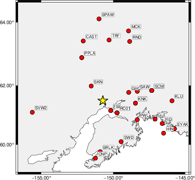
The focal mechanism was determined using broadband seismic waveforms. The location of the event (star) and the
stations used for (red) the waveform inversion are shown in the next figure.
|
|
Location of broadband stations used for waveform inversion
|
The program wvfgrd96 was used with good traces observed at short distance to determine the focal mechanism, depth and seismic moment. This technique requires a high quality signal and well determined velocity model for the Green's functions. To the extent that these are the quality data, this type of mechanism should be preferred over the radiation pattern technique which requires the separate step of defining the pressure and tension quadrants and the correct strike.
The observed and predicted traces are filtered using the following gsac commands:
hp c 0.02 n 3
lp c 0.06 n 3
The results of this grid search are as follow:
           DEPTH  STK   DIP  RAKE   MW    FIT
WVFGRD96    0.5    95    40    90   3.61 0.1719
WVFGRD96    1.0    55    60   -35   3.58 0.1703
WVFGRD96    2.0    90    45    85   3.76 0.2240
WVFGRD96    3.0    50    65   -40   3.75 0.2331
WVFGRD96    4.0    45    85   -30   3.75 0.2400
WVFGRD96    5.0    45    90   -30   3.78 0.2495
WVFGRD96    6.0   230    85    30   3.80 0.2562
WVFGRD96    7.0   230    85    30   3.81 0.2595
WVFGRD96    8.0   230    85    35   3.86 0.2615
WVFGRD96    9.0   230    85    30   3.86 0.2596
WVFGRD96   10.0    45    90    30   3.87 0.2613
WVFGRD96   11.0    50    75    35   3.88 0.2626
WVFGRD96   12.0    50    80    35   3.89 0.2654
WVFGRD96   13.0    50    80    35   3.90 0.2683
WVFGRD96   14.0    45    90    30   3.91 0.2707
WVFGRD96   15.0    45    90    30   3.92 0.2737
WVFGRD96   16.0    45    90    30   3.92 0.2765
WVFGRD96   17.0    45    90    30   3.93 0.2788
WVFGRD96   18.0    45    90    30   3.94 0.2815
WVFGRD96   19.0   225    85   -30   3.95 0.2849
WVFGRD96   20.0    50    85    30   3.96 0.2876
WVFGRD96   21.0    50    85    30   3.97 0.2912
WVFGRD96   22.0    50    90    30   3.98 0.2949
WVFGRD96   23.0   225    85   -30   3.99 0.2998
WVFGRD96   24.0   225    85   -30   4.00 0.3047
WVFGRD96   25.0   225    85   -30   4.01 0.3098
WVFGRD96   26.0   230    85   -30   4.03 0.3153
WVFGRD96   27.0    50    90    35   4.02 0.3205
WVFGRD96   28.0    50    90    35   4.03 0.3259
WVFGRD96   29.0    50    90    35   4.04 0.3316
WVFGRD96   30.0   230    85   -30   4.07 0.3380
WVFGRD96   31.0   230    85   -35   4.07 0.3435
WVFGRD96   32.0   225    80   -30   4.09 0.3495
WVFGRD96   33.0   225    80   -30   4.10 0.3554
WVFGRD96   34.0   230    80   -30   4.12 0.3605
WVFGRD96   35.0   225    80   -30   4.12 0.3648
WVFGRD96   36.0   230    80   -30   4.14 0.3691
WVFGRD96   37.0   225    75   -30   4.16 0.3729
WVFGRD96   38.0   225    75   -30   4.17 0.3757
WVFGRD96   39.0   225    75   -30   4.19 0.3782
WVFGRD96   40.0   220    70   -45   4.25 0.3841
WVFGRD96   41.0   220    70   -45   4.26 0.3894
WVFGRD96   42.0   220    70   -45   4.27 0.3937
WVFGRD96   43.0   220    65   -45   4.29 0.3991
WVFGRD96   44.0   220    65   -45   4.30 0.4039
WVFGRD96   45.0   220    65   -45   4.31 0.4093
WVFGRD96   46.0   220    65   -45   4.31 0.4135
WVFGRD96   47.0   215    65   -45   4.32 0.4186
WVFGRD96   48.0   215    65   -50   4.32 0.4228
WVFGRD96   49.0   215    65   -50   4.33 0.4277
WVFGRD96   50.0   215    65   -50   4.34 0.4315
WVFGRD96   51.0   205    60   -55   4.35 0.4365
WVFGRD96   52.0   205    60   -60   4.35 0.4401
WVFGRD96   53.0   205    60   -60   4.36 0.4443
WVFGRD96   54.0   200    60   -60   4.37 0.4477
WVFGRD96   55.0   200    60   -65   4.37 0.4510
WVFGRD96   56.0   200    60   -65   4.37 0.4546
WVFGRD96   57.0   200    60   -65   4.38 0.4570
WVFGRD96   58.0   200    60   -65   4.39 0.4597
WVFGRD96   59.0   195    60   -70   4.39 0.4615
WVFGRD96   60.0   195    60   -70   4.39 0.4637
WVFGRD96   61.0   195    60   -70   4.40 0.4651
WVFGRD96   62.0   195    60   -70   4.40 0.4655
WVFGRD96   63.0   195    60   -70   4.41 0.4663
WVFGRD96   64.0   200    65   -65   4.41 0.4666
WVFGRD96   65.0   200    65   -65   4.42 0.4673
WVFGRD96   66.0   195    65   -70   4.42 0.4673
WVFGRD96   67.0   195    65   -70   4.42 0.4672
WVFGRD96   68.0   195    65   -70   4.43 0.4672
WVFGRD96   69.0   195    65   -75   4.43 0.4669
WVFGRD96   70.0   195    65   -75   4.43 0.4656
WVFGRD96   71.0   195    65   -75   4.43 0.4650
WVFGRD96   72.0   195    65   -75   4.44 0.4634
WVFGRD96   73.0   195    65   -75   4.44 0.4614
WVFGRD96   74.0   190    65   -80   4.44 0.4596
WVFGRD96   75.0   190    65   -80   4.44 0.4576
WVFGRD96   76.0   190    65   -80   4.44 0.4550
WVFGRD96   77.0   190    65   -80   4.45 0.4532
WVFGRD96   78.0   190    65   -80   4.45 0.4503
WVFGRD96   79.0   190    65   -80   4.45 0.4470
WVFGRD96   80.0   190    65   -85   4.45 0.4446
WVFGRD96   81.0   190    65   -85   4.45 0.4414
WVFGRD96   82.0   190    65   -85   4.45 0.4377
WVFGRD96   83.0   190    70   -85   4.45 0.4345
WVFGRD96   84.0   190    70   -85   4.46 0.4329
WVFGRD96   85.0   190    70   -85   4.46 0.4300
WVFGRD96   86.0     5    20   -95   4.46 0.4268
WVFGRD96   87.0     0    20  -100   4.46 0.4245
WVFGRD96   88.0     5    20   -95   4.46 0.4214
WVFGRD96   89.0     0    20  -100   4.47 0.4182
WVFGRD96   90.0     5    20   -95   4.47 0.4155
WVFGRD96   91.0   190    70   -85   4.47 0.4120
WVFGRD96   92.0   190    70   -85   4.47 0.4083
WVFGRD96   93.0     0    20  -100   4.47 0.4044
WVFGRD96   94.0     0    20  -100   4.47 0.4011
WVFGRD96   95.0   190    70   -90   4.47 0.3971
WVFGRD96   96.0    -5    20  -105   4.48 0.3930
WVFGRD96   97.0   -10    20  -110   4.48 0.3892
WVFGRD96   98.0   -10    20  -110   4.48 0.3856
WVFGRD96   99.0     0    15  -100   4.48 0.3823
WVFGRD96  100.0     0    15  -100   4.48 0.3798
WVFGRD96  101.0   190    75   -85   4.48 0.3780
WVFGRD96  102.0     0    15  -100   4.48 0.3751
WVFGRD96  103.0    10    15   -90   4.48 0.3722
WVFGRD96  104.0    20    15   -80   4.48 0.3680
WVFGRD96  105.0   190    75   -85   4.49 0.3674
WVFGRD96  106.0   190    75   -85   4.49 0.3654
WVFGRD96  107.0   190    75   -85   4.49 0.3630
WVFGRD96  108.0   190    75   -85   4.49 0.3601
WVFGRD96  109.0   190    75   -85   4.49 0.3573
WVFGRD96  110.0   190    75   -85   4.49 0.3554
WVFGRD96  111.0   190    80   -80   4.49 0.3533
WVFGRD96  112.0   190    80   -80   4.50 0.3517
WVFGRD96  113.0   190    80   -80   4.50 0.3498
WVFGRD96  114.0   190    80   -80   4.50 0.3485
WVFGRD96  115.0   190    80   -80   4.50 0.3471
WVFGRD96  116.0   190    80   -80   4.50 0.3457
WVFGRD96  117.0   190    80   -80   4.50 0.3437
WVFGRD96  118.0   190    80   -80   4.50 0.3416
WVFGRD96  119.0   190    80   -80   4.51 0.3406
WVFGRD96  120.0   190    80   -80   4.51 0.3394
WVFGRD96  121.0   190    80   -80   4.51 0.3373
WVFGRD96  122.0   190    80   -80   4.51 0.3352
WVFGRD96  123.0   190    80   -80   4.51 0.3339
WVFGRD96  124.0   195    85   -80   4.52 0.3326
WVFGRD96  125.0   195    85   -80   4.52 0.3316
WVFGRD96  126.0   195    85   -80   4.52 0.3305
WVFGRD96  127.0   195    85   -80   4.53 0.3291
WVFGRD96  128.0   195    85   -80   4.53 0.3283
WVFGRD96  129.0   195    85   -80   4.53 0.3274
The best solution is
WVFGRD96 66.0 195 65 -70 4.42 0.4673
The mechanism corresponding to the best fit is
|
|
Figure 1. Waveform inversion focal mechanism
|
The best fit as a function of depth is given in the following figure:
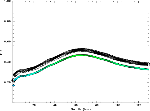
|
|
Figure 2. Depth sensitivity for waveform mechanism
|
The comparison of the observed and predicted waveforms is given in the next figure. The red traces are the observed and the blue are the predicted.
Each observed-predicted component is plotted to the same scale and peak amplitudes are indicated by the numbers to the left of each trace. A pair of numbers is given in black at the right of each predicted traces. The upper number it the time shift required for maximum correlation between the observed and predicted traces. This time shift is required because the synthetics are not computed at exactly the same distance as the observed, the velocity model used in the predictions may not be perfect and the epicentral parameters may be be off.
A positive time shift indicates that the prediction is too fast and should be delayed to match the observed trace (shift to the right in this figure). A negative value indicates that the prediction is too slow. The lower number gives the percentage of variance reduction to characterize the individual goodness of fit (100% indicates a perfect fit).
The bandpass filter used in the processing and for the display was
hp c 0.02 n 3
lp c 0.06 n 3

|
|
Figure 3. Waveform comparison for selected depth. Red: observed; Blue - predicted. The time shift with respect to the model prediction is indicated. The percent of fit is also indicated. The time scale is relative to the first trace sample.
|
|
|
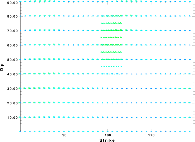
Focal mechanism sensitivity at the preferred depth. The red color indicates a very good fit to the waveforms.
Each solution is plotted as a vector at a given value of strike and dip with the angle of the vector representing the rake angle, measured, with respect to the upward vertical (N) in the figure.
|
A check on the assumed source location is possible by looking at the time shifts between the observed and predicted traces. The time shifts for waveform matching arise for several reasons:
- The origin time and epicentral distance are incorrect
- The velocity model used for the inversion is incorrect
- The velocity model used to define the P-arrival time is not the
same as the velocity model used for the waveform inversion
(assuming that the initial trace alignment is based on the
P arrival time)
Assuming only a mislocation, the time shifts are fit to a functional form:
Time_shift = A + B cos Azimuth + C Sin Azimuth
The time shifts for this inversion lead to the next figure:
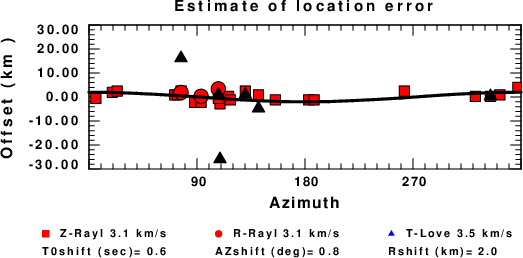
The derived shift in origin time and epicentral coordinates are given at the bottom of the figure.
Velocity Model
The WUS.model used for the waveform synthetic seismograms and for the surface wave eigenfunctions and dispersion is as follows
(The format is in the model96 format of Computer Programs in Seismology).
MODEL.01
Model after     8 iterations
ISOTROPIC
KGS
FLAT EARTH
1-D
CONSTANT VELOCITY
LINE08
LINE09
LINE10
LINE11
      H(KM)   VP(KM/S)   VS(KM/S) RHO(GM/CC)         QP         QS       ETAP       ETAS      FREFP      FREFS
     1.9000     3.4065     2.0089     2.2150  0.302E-02  0.679E-02   0.00       0.00       1.00       1.00
     6.1000     5.5445     3.2953     2.6089  0.349E-02  0.784E-02   0.00       0.00       1.00       1.00
    13.0000     6.2708     3.7396     2.7812  0.212E-02  0.476E-02   0.00       0.00       1.00       1.00
    19.0000     6.4075     3.7680     2.8223  0.111E-02  0.249E-02   0.00       0.00       1.00       1.00
     0.0000     7.9000     4.6200     3.2760  0.164E-10  0.370E-10   0.00       0.00       1.00       1.00
Last Changed Fri Apr 26 11:38:03 PM CDT 2024