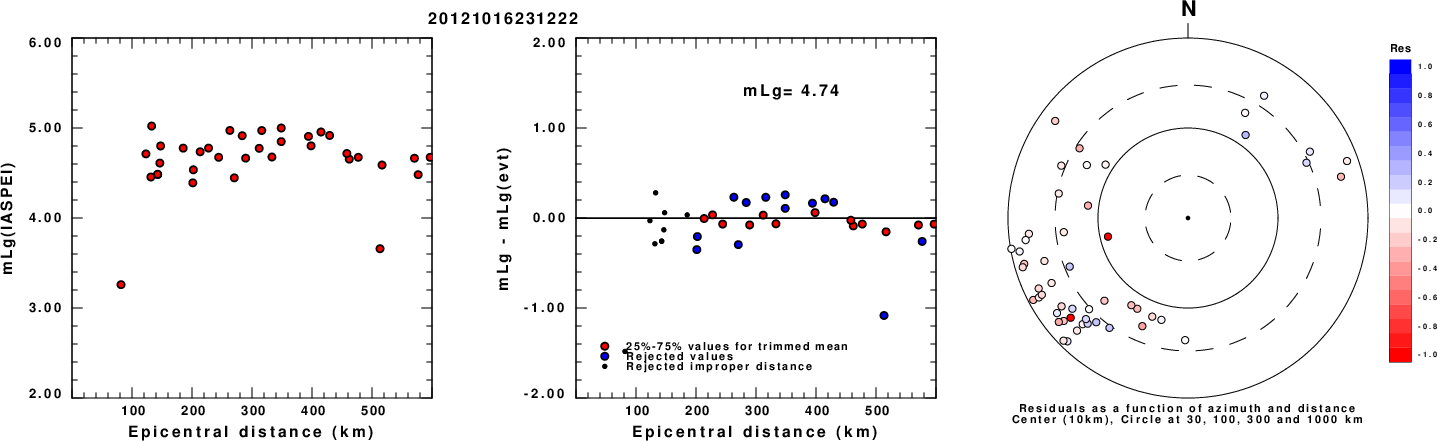
Left: mLg computed using the IASPEI formula. Center: mLg residuals versus epicentral distance ; the values used for the trimmed mean magnitude estimate are indicated. Right: residuals as a function of distance and azimuth.
The ANSS event ID is ld60036706 and the event page is at https://earthquake.usgs.gov/earthquakes/eventpage/ld60036706/executive.
2012/10/16 23:12:22 43.597 -70.656 16.1 4.67 Maine
 USGS/SLU Moment Tensor Solution
 ENS  2012/10/16 23:12:22:0  43.60  -70.66  16.1 4.7 Maine

 Stations used:
   CN.A16 CN.A21 CN.A54 CN.A61 CN.A64 CN.ALFO CN.ALGO CN.BANO
   CN.DELO CN.DMCQ CN.DRCO CN.GAC CN.GGN CN.HAL CN.KGNO CN.LMQ
   CN.MEDO CN.MNTQ CN.ORHO CN.ORIO CN.OTT CN.PEMO CN.PKRO
   CN.PLVO CN.SADO CN.STCO IU.HRV LD.ACCN LD.BRNJ LD.FRNY
   LD.KSCT LD.KSPA LD.MMNY LD.NCB LD.ODNJ LD.PAL NE.BCX
   NE.BRYW NE.EMMW NE.PQI NE.QUA2 NE.TRY NE.VT1 NE.WES NE.WSPT
   NE.WVL NE.YLE PE.PSUB TA.M65A TA.N59A US.BINY US.LBNH
   US.LONY US.PKME

 Filtering commands used:
   hp c 0.02 n 3
   lp c 0.10 n 3

 Best Fitting Double Couple
  Mo = 1.40e+22 dyne-cm
  Mw = 4.03
  Z  = 7 km
  Plane   Strike  Dip  Rake
   NP1      348    61    84
   NP2      180    30   100
  Principal Axes:
   Axis    Value   Plunge  Azimuth
    T   1.40e+22     74     244
    N   0.00e+00      5     351
    P  -1.40e+22     15      83

 Moment Tensor: (dyne-cm)
    Component   Value
       Mxx     2.12e+14
       Mxy    -1.21e+21
       Mxz    -2.10e+21
       Myy    -1.19e+22
       Myz    -6.88e+21
       Mzz     1.19e+22


                     --------------
                 -----#####------------
              ------#########-------------
             -----############-------------
           ------###############-------------
          ------################--------------
         ------##################--------------
        ------####################--------------
        ------#####################---------   -
       ------######################--------- P --
       ------######################---------   --
       ------########   ############-------------
       ------######## T ############-------------
        ------#######   ############------------
        ------######################------------
         ------#####################-----------
          ------####################----------
           ------###################---------
             -----#################--------
              ------###############-------
                 -----############-----
                     ----########--


 Global CMT Convention Moment Tensor:
      R          T          P
  1.19e+22  -2.10e+21   6.88e+21
 -2.10e+21   2.12e+14   1.21e+21
  6.88e+21   1.21e+21  -1.19e+22


Details of the solution is found at

http://www.eas.slu.edu/eqc/eqc_mt/MECH.NA/20121016231222/index.html
|
      STK = 180
      DIP = 30
     RAKE = 100
       MW = 4.03
       HS = 7.0
The NDK file is 20121016231222.ndk The waveform inversion is preferred.
Given the availability of digital waveforms for determination of the moment tensor, this section documents the added processing leading to mLg, if appropriate to the region, and ML by application of the respective IASPEI formulae. As a research study, the linear distance term of the IASPEI formula for ML is adjusted to remove a linear distance trend in residuals to give a regionally defined ML. The defined ML uses horizontal component recordings, but the same procedure is applied to the vertical components since there may be some interest in vertical component ground motions. Residual plots versus distance may indicate interesting features of ground motion scaling in some distance ranges. A residual plot of the regionalized magnitude is given as a function of distance and azimuth, since data sets may transcend different wave propagation provinces.
Left: mLg computed using the IASPEI formula. Center: mLg residuals versus epicentral distance ; the values used for the trimmed mean magnitude estimate are indicated.
Right: residuals as a function of distance and azimuth.
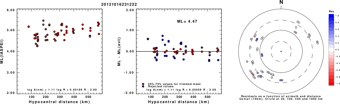
Left: ML computed using the IASPEI formula for Horizontal components. Center: ML residuals computed using a modified IASPEI formula that accounts for path specific attenuation; the values used for the trimmed mean are indicated. The ML relation used for each figure is given at the bottom of each plot.
Right: Residuals from new relation as a function of distance and azimuth.
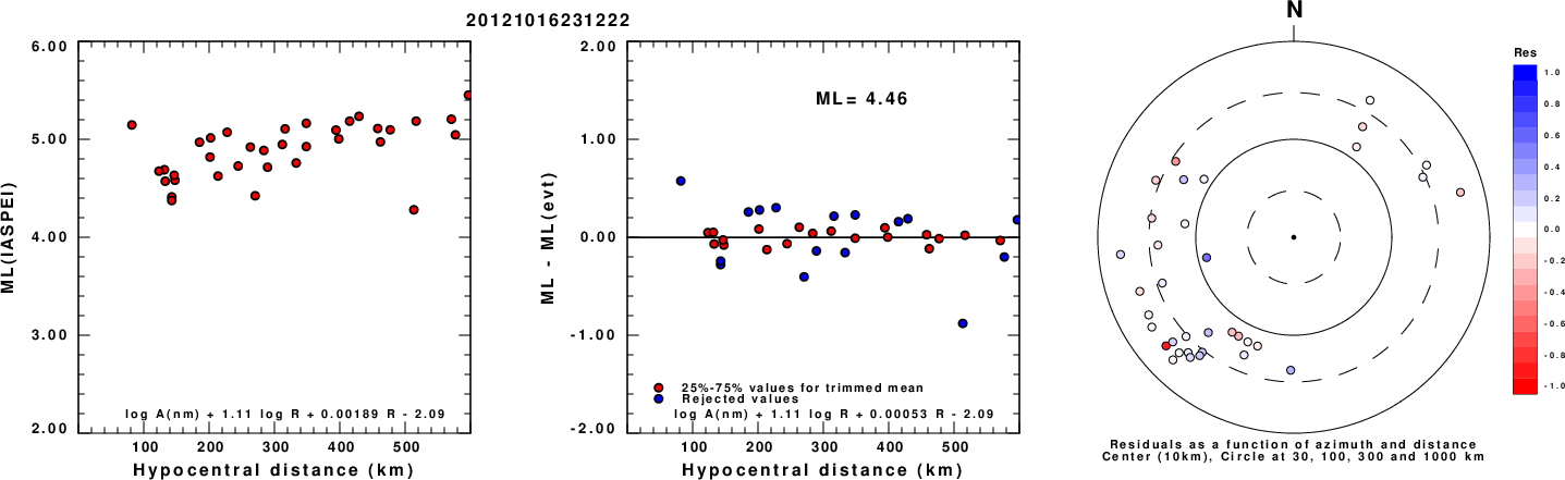
Left: ML computed using the IASPEI formula for Vertical components (research). Center: ML residuals computed using a modified IASPEI formula that accounts for path specific attenuation; the values used for the trimmed mean are indicated. The ML relation used for each figure is given at the bottom of each plot.
Right: Residuals from new relation as a function of distance and azimuth.
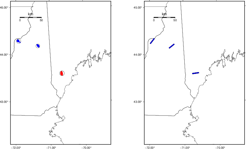 |
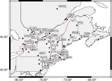
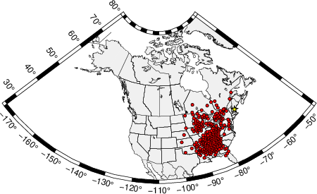
The focal mechanism was determined using broadband seismic waveforms. The location of the event (star) and the stations used for (red) the waveform inversion are shown in the next figure.
|
|
|
The program wvfgrd96 was used with good traces observed at short distance to determine the focal mechanism, depth and seismic moment. This technique requires a high quality signal and well determined velocity model for the Green's functions. To the extent that these are the quality data, this type of mechanism should be preferred over the radiation pattern technique which requires the separate step of defining the pressure and tension quadrants and the correct strike.
The observed and predicted traces are filtered using the following gsac commands:
hp c 0.02 n 3
lp c 0.10 n 3
The results of this grid search are as follow:
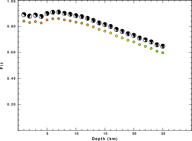
           DEPTH  STK   DIP  RAKE   MW    FIT
WVFGRD96    0.5   145    90   -75   4.17 0.5055
WVFGRD96    1.0   145    90   -75   4.17 0.5138
WVFGRD96    2.0   330    85    65   4.03 0.5640
WVFGRD96    3.0   340    75    75   4.01 0.5985
WVFGRD96    4.0   345    70    80   4.01 0.6472
WVFGRD96    5.0   350    65    85   4.03 0.6857
WVFGRD96    6.0   350    60    85   4.04 0.7049
WVFGRD96    7.0   180    30   100   4.03 0.7094
WVFGRD96    8.0   345    60    85   4.02 0.7010
WVFGRD96    9.0   165    30    90   4.02 0.6848
WVFGRD96   10.0   345    60    85   4.04 0.6711
WVFGRD96   11.0   345    60    85   4.04 0.6482
WVFGRD96   12.0   340    60    75   4.03 0.6240
WVFGRD96   13.0   335    60    70   4.03 0.5993
WVFGRD96   14.0   335    60    65   4.03 0.5758
WVFGRD96   15.0   335    60    65   4.04 0.5515
WVFGRD96   16.0   330    60    60   4.04 0.5279
WVFGRD96   17.0   330    60    60   4.04 0.5045
WVFGRD96   18.0   330    60    60   4.04 0.4814
WVFGRD96   19.0   325    65    55   4.04 0.4587
WVFGRD96   20.0   325    65    55   4.07 0.4401
WVFGRD96   21.0   325    65    55   4.07 0.4198
WVFGRD96   22.0   325    65    55   4.08 0.3994
WVFGRD96   23.0   325    65    50   4.08 0.3802
WVFGRD96   24.0   325    65    50   4.08 0.3617
WVFGRD96   25.0   320    65    50   4.08 0.3446
WVFGRD96   26.0   320    65    50   4.09 0.3302
WVFGRD96   27.0   320    65    50   4.09 0.3160
WVFGRD96   28.0   320    65    50   4.09 0.3028
WVFGRD96   29.0   100    70   -45   4.11 0.2907
The best solution is
WVFGRD96 7.0 180 30 100 4.03 0.7094
The mechanism corresponding to the best fit is
|
|
|
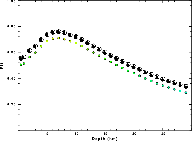
The best fit as a function of depth is given in the following figure:
|
|
|
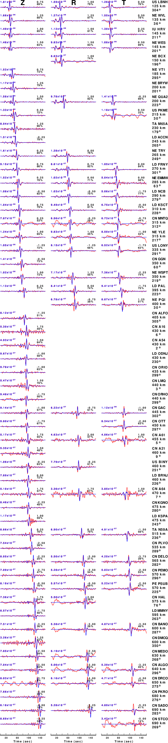
The comparison of the observed and predicted waveforms is given in the next figure. The red traces are the observed and the blue are the predicted. Each observed-predicted component is plotted to the same scale and peak amplitudes are indicated by the numbers to the left of each trace. A pair of numbers is given in black at the right of each predicted traces. The upper number it the time shift required for maximum correlation between the observed and predicted traces. This time shift is required because the synthetics are not computed at exactly the same distance as the observed, the velocity model used in the predictions may not be perfect and the epicentral parameters may be be off. A positive time shift indicates that the prediction is too fast and should be delayed to match the observed trace (shift to the right in this figure). A negative value indicates that the prediction is too slow. The lower number gives the percentage of variance reduction to characterize the individual goodness of fit (100% indicates a perfect fit).
The bandpass filter used in the processing and for the display was
hp c 0.02 n 3
lp c 0.10 n 3
|
| Figure 3. Waveform comparison for selected depth. Red: observed; Blue - predicted. The time shift with respect to the model prediction is indicated. The percent of fit is also indicated. The time scale is relative to the first trace sample. |
|
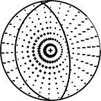
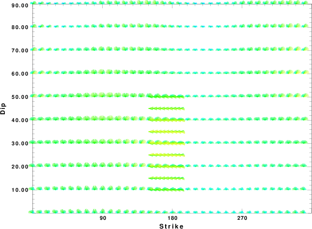
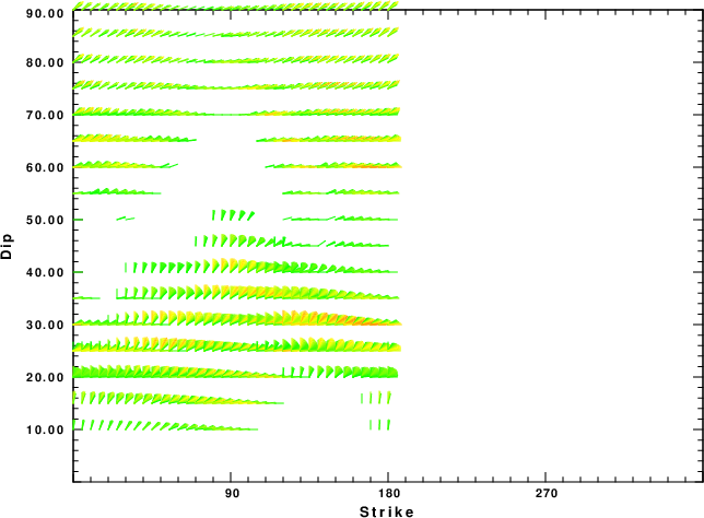
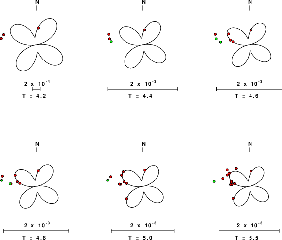
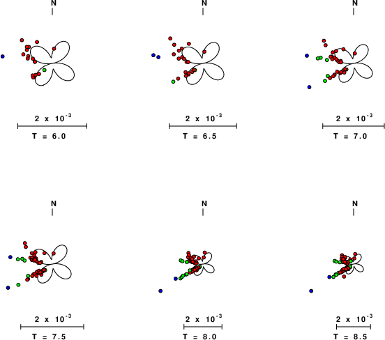
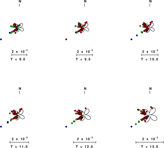
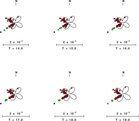
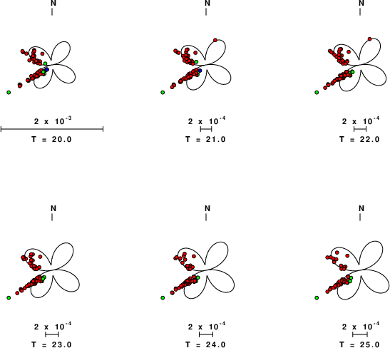
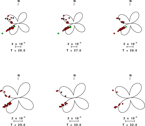
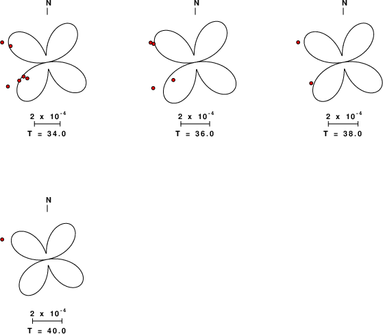
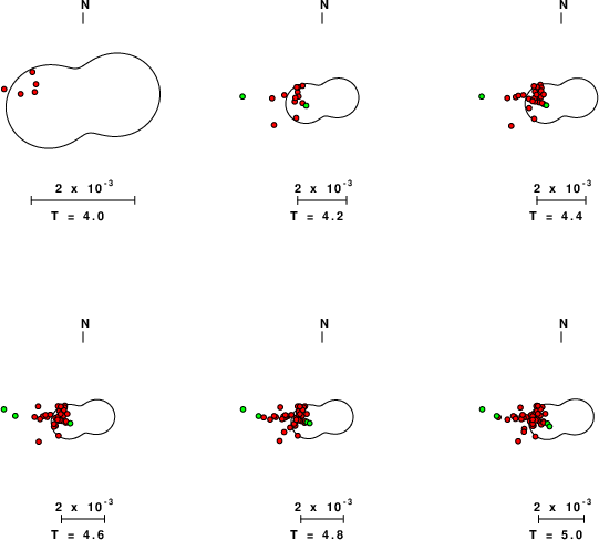
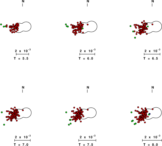
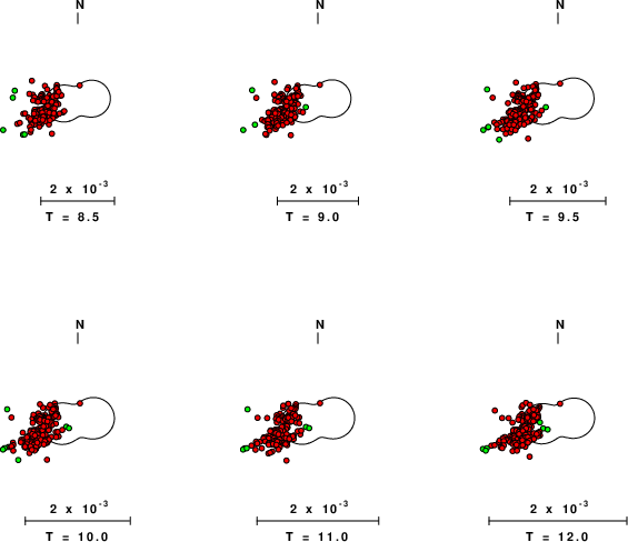
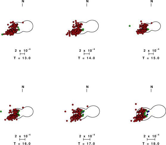
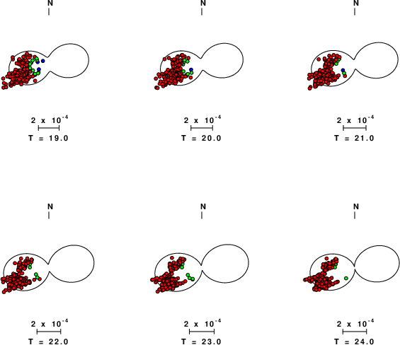
| Focal mechanism sensitivity at the preferred depth. The red color indicates a very good fit to the waveforms. Each solution is plotted as a vector at a given value of strike and dip with the angle of the vector representing the rake angle, measured, with respect to the upward vertical (N) in the figure. |
A check on the assumed source location is possible by looking at the time shifts between the observed and predicted traces. The time shifts for waveform matching arise for several reasons:
Time_shift = A + B cos Azimuth + C Sin Azimuth
The time shifts for this inversion lead to the next figure:
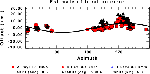
The derived shift in origin time and epicentral coordinates are given at the bottom of the figure.
The following figure shows the stations used in the grid search for the best focal mechanism to fit the surface-wave spectral amplitudes of the Love and Rayleigh waves.
|
|
|
The surface-wave determined focal mechanism is shown here.
  NODAL PLANES


  STK=     350.00
  DIP=      60.00
 RAKE=      90.00

             OR

  STK=     170.00
  DIP=      30.00
 RAKE=      90.00


DEPTH = 6.0 km

Mw = 4.16
Best Fit 0.8591 - P-T axis plot gives solutions with FIT greater than FIT90
 |
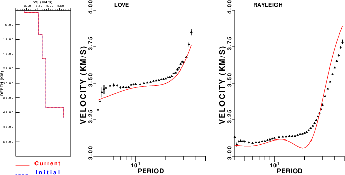
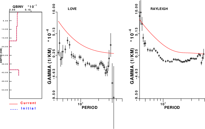
Surface wave analysis was performed using codes from Computer Programs in Seismology, specifically the multiple filter analysis program do_mft and the surface-wave radiation pattern search program srfgrd96.
Digital data were collected, instrument response removed and traces converted
to Z, R an T components. Multiple filter analysis was applied to the Z and T traces to obtain the Rayleigh- and Love-wave spectral amplitudes, respectively.
These were input to the search program which examined all depths between 1 and 25 km
and all possible mechanisms.
|
|
|

|
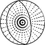
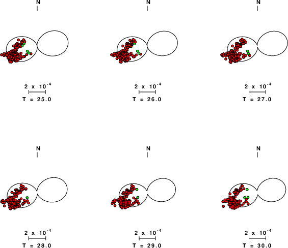
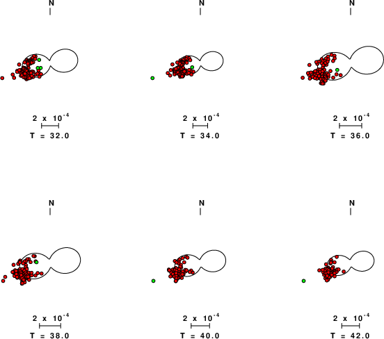
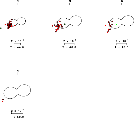
| Pressure-tension axis trends. Since the surface-wave spectra search does not distinguish between P and T axes and since there is a 180 ambiguity in strike, all possible P and T axes are plotted. First motion data and waveforms will be used to select the preferred mechanism. The purpose of this plot is to provide an idea of the possible range of solutions. The P and T-axes for all mechanisms with goodness of fit greater than 0.9 FITMAX (above) are plotted here. |
|
| Focal mechanism sensitivity at the preferred depth. The red color indicates a very good fit to the Love and Rayleigh wave radiation patterns. Each solution is plotted as a vector at a given value of strike and dip with the angle of the vector representing the rake angle, measured, with respect to the upward vertical (N) in the figure. Because of the symmetry of the spectral amplitude rediation patterns, only strikes from 0-180 degrees are sampled. |
|
|
The WUS.model used for the waveform synthetic seismograms and for the surface wave eigenfunctions and dispersion is as follows (The format is in the model96 format of Computer Programs in Seismology).
MODEL.01
Model after     8 iterations
ISOTROPIC
KGS
FLAT EARTH
1-D
CONSTANT VELOCITY
LINE08
LINE09
LINE10
LINE11
      H(KM)   VP(KM/S)   VS(KM/S) RHO(GM/CC)         QP         QS       ETAP       ETAS      FREFP      FREFS
     1.9000     3.4065     2.0089     2.2150  0.302E-02  0.679E-02   0.00       0.00       1.00       1.00
     6.1000     5.5445     3.2953     2.6089  0.349E-02  0.784E-02   0.00       0.00       1.00       1.00
    13.0000     6.2708     3.7396     2.7812  0.212E-02  0.476E-02   0.00       0.00       1.00       1.00
    19.0000     6.4075     3.7680     2.8223  0.111E-02  0.249E-02   0.00       0.00       1.00       1.00
     0.0000     7.9000     4.6200     3.2760  0.164E-10  0.370E-10   0.00       0.00       1.00       1.00