Location
Location ANSS
The ANSS event ID is ak012c1bnwdr and the event page is at
https://earthquake.usgs.gov/earthquakes/eventpage/ak012c1bnwdr/executive.
2012/09/18 01:44:49 56.937 -154.142 38.6 5.2 Alaska
Focal Mechanism
 USGS/SLU Moment Tensor Solution
 ENS  2012/09/18 01:44:49:0  56.94 -154.14  38.6 5.2 Alaska

 Stations used:
   AK.BMR AK.BPAW AK.BRLK AK.CAST AK.CNP AK.DHY AK.DIV AK.EYAK
   AK.FALS AK.FID AK.GLI AK.HOM AK.KLU AK.KNK AK.KTH AK.MCK
   AK.PPLA AK.PWL AK.RC01 AK.RND AK.SAW AK.SCM AK.SKN AK.TRF
   AK.UNV AT.AKUT AT.CHGN AT.OHAK AT.SDPT AT.SVW2 II.KDAK

 Filtering commands used:
   hp c 0.02 n 3
   lp c 0.04 n 3

 Best Fitting Double Couple
  Mo = 5.25e+23 dyne-cm
  Mw = 5.08
  Z  = 42 km
  Plane   Strike  Dip  Rake
   NP1      142    86   -150
   NP2       50    60    -5
  Principal Axes:
   Axis    Value   Plunge  Azimuth
    T   5.25e+23     17     272
    N   0.00e+00     60     150
    P  -5.25e+23     24      10

 Moment Tensor: (dyne-cm)
    Component   Value
       Mxx    -4.23e+23
       Mxy    -9.81e+22
       Mxz    -1.86e+23
       Myy     4.62e+23
       Myz    -1.86e+23
       Mzz    -3.96e+22


                     --------------
                 ------------   -------
              ##------------- P ----------
             ####------------   -----------
           #######--------------------------#
          #########-------------------------##
         ############----------------------####
        ##############--------------------######
        ###############------------------#######
       ##   #############---------------#########
       ## T ##############-------------##########
       ##   ###############-----------###########
       ######################-------#############
        ######################----##############
        ########################################
         #####################---##############
          #################--------###########
           ###########--------------#########
             -------------------------#####
              --------------------------##
                 ----------------------
                     --------------


 Global CMT Convention Moment Tensor:
      R          T          P
 -3.96e+22  -1.86e+23   1.86e+23
 -1.86e+23  -4.23e+23   9.81e+22
  1.86e+23   9.81e+22   4.62e+23


Details of the solution is found at

http://www.eas.slu.edu/eqc/eqc_mt/MECH.NA/20120918014449/index.html
|
Preferred Solution
The preferred solution from an analysis of the surface-wave spectral amplitude radiation pattern, waveform inversion or first motion observations is
      STK = 50
      DIP = 60
     RAKE = -5
       MW = 5.08
       HS = 42.0
The NDK file is 20120918014449.ndk
The waveform inversion is preferred.
Moment Tensor Comparison
The following compares this source inversion to those provided by others. The purpose is to look for major differences and also to note slight differences that might be inherent to the processing procedure. For completeness the USGS/SLU solution is repeated from above.
| SLU |
GCMT |
 USGS/SLU Moment Tensor Solution
 ENS  2012/09/18 01:44:49:0  56.94 -154.14  38.6 5.2 Alaska

 Stations used:
   AK.BMR AK.BPAW AK.BRLK AK.CAST AK.CNP AK.DHY AK.DIV AK.EYAK
   AK.FALS AK.FID AK.GLI AK.HOM AK.KLU AK.KNK AK.KTH AK.MCK
   AK.PPLA AK.PWL AK.RC01 AK.RND AK.SAW AK.SCM AK.SKN AK.TRF
   AK.UNV AT.AKUT AT.CHGN AT.OHAK AT.SDPT AT.SVW2 II.KDAK

 Filtering commands used:
   hp c 0.02 n 3
   lp c 0.04 n 3

 Best Fitting Double Couple
  Mo = 5.25e+23 dyne-cm
  Mw = 5.08
  Z  = 42 km
  Plane   Strike  Dip  Rake
   NP1      142    86   -150
   NP2       50    60    -5
  Principal Axes:
   Axis    Value   Plunge  Azimuth
    T   5.25e+23     17     272
    N   0.00e+00     60     150
    P  -5.25e+23     24      10

 Moment Tensor: (dyne-cm)
    Component   Value
       Mxx    -4.23e+23
       Mxy    -9.81e+22
       Mxz    -1.86e+23
       Myy     4.62e+23
       Myz    -1.86e+23
       Mzz    -3.96e+22


                     --------------
                 ------------   -------
              ##------------- P ----------
             ####------------   -----------
           #######--------------------------#
          #########-------------------------##
         ############----------------------####
        ##############--------------------######
        ###############------------------#######
       ##   #############---------------#########
       ## T ##############-------------##########
       ##   ###############-----------###########
       ######################-------#############
        ######################----##############
        ########################################
         #####################---##############
          #################--------###########
           ###########--------------#########
             -------------------------#####
              --------------------------##
                 ----------------------
                     --------------


 Global CMT Convention Moment Tensor:
      R          T          P
 -3.96e+22  -1.86e+23   1.86e+23
 -1.86e+23  -4.23e+23   9.81e+22
  1.86e+23   9.81e+22   4.62e+23


Details of the solution is found at

http://www.eas.slu.edu/eqc/eqc_mt/MECH.NA/20120918014449/index.html
|
Global CMT Project Moment Tensor Solution


September 18, 2012, KODIAK ISLAND REGION, ALASKA, MW=5.2

Howard Koss

CENTROID-MOMENT-TENSOR  SOLUTION
GCMT EVENT:     C201209180144A
DATA: II IU CU MN LD G  IC DK GE
L.P.BODY WAVES: 72S, 104C, T= 40
SURFACE WAVES: 115S, 185C, T= 50
TIMESTAMP:      Q-20120918053847
CENTROID LOCATION:
ORIGIN TIME:      01:44:49.8 0.2
LAT:56.96N 0.02;LON:154.30W 0.02
DEP: 30.7  1.0;TRIANG HDUR:  1.0
MOMENT TENSOR: SCALE 10**23 D-CM
RR=-2.770 0.174; TT=-3.040 0.159
PP= 5.810 0.145; RT= 3.640 0.233
RP= 4.830 0.218; TP= 2.600 0.103
PRINCIPAL AXES:
1.(T) VAL=  9.233;PLG=26;AZM=290
2.(N)      -2.440;    29;     35
3.(P)      -6.793;    50;    165
BEST DBLE.COUPLE:M0= 8.01*10**23
NP1: STRIKE=335;DIP=32;SLIP=-154
NP2: STRIKE=223;DIP=77;SLIP= -60

            -----------
        ###########--------
      ################------#
    ####################-######
   ###################----######
  ##   #############-------######
  ## T ###########----------#####
 ###   #########-------------#####
 ##############--------------#####
 ############----------------#####
 ###########-----------------#####
  ########-------------------####
  #######---------   --------####
   #####---------- P --------###
    ###-----------   -------###
      ---------------------##
        ------------------#
            -----------
|
Magnitudes
Given the availability of digital waveforms for determination of the moment tensor, this section documents the added processing leading to mLg, if appropriate to the region, and ML by application of the respective IASPEI formulae. As a research study, the linear distance term of the IASPEI formula
for ML is adjusted to remove a linear distance trend in residuals to give a regionally defined ML. The defined ML uses horizontal component recordings, but the same procedure is applied to the vertical components since there may be some interest in vertical component ground motions. Residual plots versus distance may indicate interesting features of ground motion scaling in some distance ranges. A residual plot of the regionalized magnitude is given as a function of distance and azimuth, since data sets may transcend different wave propagation provinces.
ML Magnitude
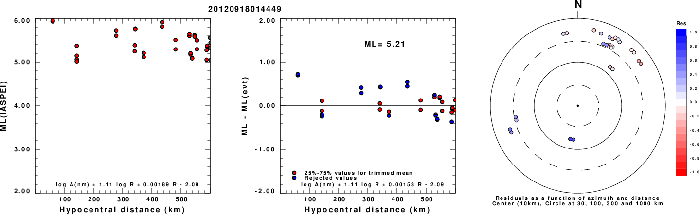
Left: ML computed using the IASPEI formula for Horizontal components. Center: ML residuals computed using a modified IASPEI formula that accounts for path specific attenuation; the values used for the trimmed mean are indicated. The ML relation used for each figure is given at the bottom of each plot.
Right: Residuals from new relation as a function of distance and azimuth.
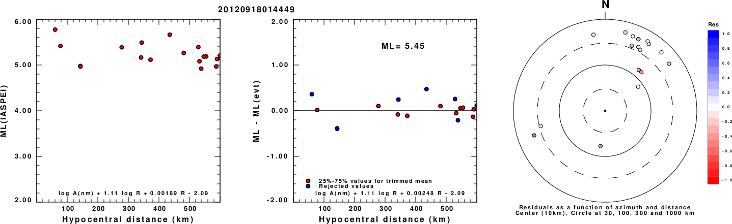
Left: ML computed using the IASPEI formula for Vertical components (research). Center: ML residuals computed using a modified IASPEI formula that accounts for path specific attenuation; the values used for the trimmed mean are indicated. The ML relation used for each figure is given at the bottom of each plot.
Right: Residuals from new relation as a function of distance and azimuth.
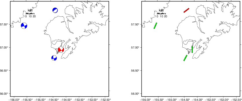
Context
The left panel of the next figure presents the focal mechanism for this earthquake (red) in the context of other nearby events (blue) in the SLU Moment Tensor Catalog. The right panel shows the inferred direction of maximum compressive stress and the type of faulting (green is strike-slip, red is normal, blue is thrust; oblique is shown by a combination of colors). Thus context plot is useful for assessing the appropriateness of the moment tensor of this event.
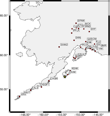
Waveform Inversion using wvfgrd96
The focal mechanism was determined using broadband seismic waveforms. The location of the event (star) and the
stations used for (red) the waveform inversion are shown in the next figure.
|
|
Location of broadband stations used for waveform inversion
|
The program wvfgrd96 was used with good traces observed at short distance to determine the focal mechanism, depth and seismic moment. This technique requires a high quality signal and well determined velocity model for the Green's functions. To the extent that these are the quality data, this type of mechanism should be preferred over the radiation pattern technique which requires the separate step of defining the pressure and tension quadrants and the correct strike.
The observed and predicted traces are filtered using the following gsac commands:
hp c 0.02 n 3
lp c 0.04 n 3
The results of this grid search are as follow:
           DEPTH  STK   DIP  RAKE   MW    FIT
WVFGRD96    0.5   190    45    80   4.62 0.3181
WVFGRD96    1.0   105    90     5   4.50 0.3342
WVFGRD96    2.0   190    45    90   4.69 0.3974
WVFGRD96    3.0   115    65    30   4.62 0.4228
WVFGRD96    4.0   290    60    20   4.66 0.4384
WVFGRD96    5.0   290    65    20   4.68 0.4418
WVFGRD96    6.0   105    75    10   4.69 0.4389
WVFGRD96    7.0   285    75    10   4.71 0.4335
WVFGRD96    8.0    65    55    10   4.75 0.4346
WVFGRD96    9.0    65    55    15   4.76 0.4565
WVFGRD96   10.0    60    55    10   4.76 0.4739
WVFGRD96   11.0    60    55    10   4.77 0.4903
WVFGRD96   12.0    60    55    10   4.78 0.5054
WVFGRD96   13.0    60    55    15   4.78 0.5190
WVFGRD96   14.0    60    60    10   4.80 0.5314
WVFGRD96   15.0    60    60    10   4.80 0.5437
WVFGRD96   16.0    55    60     5   4.80 0.5557
WVFGRD96   17.0    55    60     5   4.81 0.5685
WVFGRD96   18.0    55    60     5   4.82 0.5793
WVFGRD96   19.0    55    60     5   4.82 0.5892
WVFGRD96   20.0    55    60     5   4.83 0.5993
WVFGRD96   21.0    50    60     0   4.84 0.6085
WVFGRD96   22.0    50    60    -5   4.85 0.6188
WVFGRD96   23.0    50    60    -5   4.86 0.6280
WVFGRD96   24.0    50    60    -5   4.87 0.6365
WVFGRD96   25.0    50    60    -5   4.87 0.6450
WVFGRD96   26.0    50    60    -5   4.88 0.6519
WVFGRD96   27.0    50    60    -5   4.89 0.6584
WVFGRD96   28.0    50    60    -5   4.90 0.6648
WVFGRD96   29.0    50    60   -10   4.91 0.6697
WVFGRD96   30.0    50    65    -5   4.93 0.6748
WVFGRD96   31.0    50    65    -5   4.93 0.6802
WVFGRD96   32.0    50    65     0   4.94 0.6846
WVFGRD96   33.0    50    65     0   4.95 0.6892
WVFGRD96   34.0    50    65     0   4.95 0.6930
WVFGRD96   35.0    50    65     0   4.96 0.6965
WVFGRD96   36.0    50    70    10   4.98 0.7001
WVFGRD96   37.0    50    70    10   4.99 0.7062
WVFGRD96   38.0    50    70    10   5.00 0.7123
WVFGRD96   39.0    50    70    10   5.01 0.7181
WVFGRD96   40.0    50    60    -5   5.06 0.7188
WVFGRD96   41.0    50    60    -5   5.07 0.7199
WVFGRD96   42.0    50    60    -5   5.08 0.7200
WVFGRD96   43.0    50    60    -5   5.08 0.7193
WVFGRD96   44.0    50    60    -5   5.09 0.7180
WVFGRD96   45.0    50    60    -5   5.09 0.7160
WVFGRD96   46.0    50    60    -5   5.10 0.7135
WVFGRD96   47.0    50    60    -5   5.10 0.7104
WVFGRD96   48.0    50    65     0   5.11 0.7075
WVFGRD96   49.0    50    65     5   5.11 0.7048
The best solution is
WVFGRD96 42.0 50 60 -5 5.08 0.7200
The mechanism corresponding to the best fit is
|
|
Figure 1. Waveform inversion focal mechanism
|
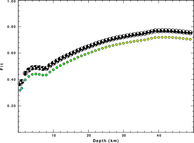
The best fit as a function of depth is given in the following figure:
|
|
Figure 2. Depth sensitivity for waveform mechanism
|
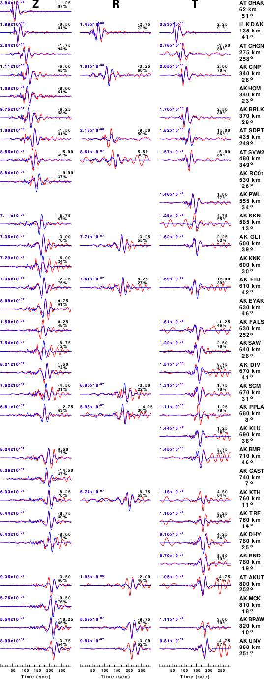
The comparison of the observed and predicted waveforms is given in the next figure. The red traces are the observed and the blue are the predicted.
Each observed-predicted component is plotted to the same scale and peak amplitudes are indicated by the numbers to the left of each trace. A pair of numbers is given in black at the right of each predicted traces. The upper number it the time shift required for maximum correlation between the observed and predicted traces. This time shift is required because the synthetics are not computed at exactly the same distance as the observed, the velocity model used in the predictions may not be perfect and the epicentral parameters may be be off.
A positive time shift indicates that the prediction is too fast and should be delayed to match the observed trace (shift to the right in this figure). A negative value indicates that the prediction is too slow. The lower number gives the percentage of variance reduction to characterize the individual goodness of fit (100% indicates a perfect fit).
The bandpass filter used in the processing and for the display was
hp c 0.02 n 3
lp c 0.04 n 3
|
|
Figure 3. Waveform comparison for selected depth. Red: observed; Blue - predicted. The time shift with respect to the model prediction is indicated. The percent of fit is also indicated. The time scale is relative to the first trace sample.
|
|
|
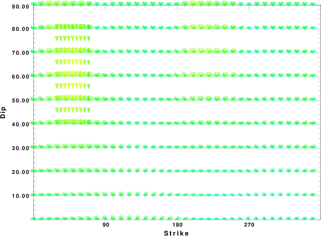
Focal mechanism sensitivity at the preferred depth. The red color indicates a very good fit to the waveforms.
Each solution is plotted as a vector at a given value of strike and dip with the angle of the vector representing the rake angle, measured, with respect to the upward vertical (N) in the figure.
|
A check on the assumed source location is possible by looking at the time shifts between the observed and predicted traces. The time shifts for waveform matching arise for several reasons:
- The origin time and epicentral distance are incorrect
- The velocity model used for the inversion is incorrect
- The velocity model used to define the P-arrival time is not the
same as the velocity model used for the waveform inversion
(assuming that the initial trace alignment is based on the
P arrival time)
Assuming only a mislocation, the time shifts are fit to a functional form:
Time_shift = A + B cos Azimuth + C Sin Azimuth
The time shifts for this inversion lead to the next figure:
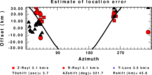
The derived shift in origin time and epicentral coordinates are given at the bottom of the figure.
Velocity Model
The WUS.model used for the waveform synthetic seismograms and for the surface wave eigenfunctions and dispersion is as follows
(The format is in the model96 format of Computer Programs in Seismology).
MODEL.01
Model after     8 iterations
ISOTROPIC
KGS
FLAT EARTH
1-D
CONSTANT VELOCITY
LINE08
LINE09
LINE10
LINE11
      H(KM)   VP(KM/S)   VS(KM/S) RHO(GM/CC)         QP         QS       ETAP       ETAS      FREFP      FREFS
     1.9000     3.4065     2.0089     2.2150  0.302E-02  0.679E-02   0.00       0.00       1.00       1.00
     6.1000     5.5445     3.2953     2.6089  0.349E-02  0.784E-02   0.00       0.00       1.00       1.00
    13.0000     6.2708     3.7396     2.7812  0.212E-02  0.476E-02   0.00       0.00       1.00       1.00
    19.0000     6.4075     3.7680     2.8223  0.111E-02  0.249E-02   0.00       0.00       1.00       1.00
     0.0000     7.9000     4.6200     3.2760  0.164E-10  0.370E-10   0.00       0.00       1.00       1.00
Last Changed Fri Apr 26 11:11:21 PM CDT 2024