Location
Location ANSS
The ANSS event ID is ak012b4fi0t8 and the event page is at
https://earthquake.usgs.gov/earthquakes/eventpage/ak012b4fi0t8/executive.
2012/08/29 12:50:55 60.334 -150.735 65.8 4.4 Alaska
Focal Mechanism
 USGS/SLU Moment Tensor Solution
 ENS  2012/08/29 12:50:55:0  60.33 -150.74  65.8 4.4 Alaska

 Stations used:
   AK.BMR AK.BPAW AK.BRLK AK.CNP AK.DOT AK.FIB AK.FID AK.GHO
   AK.GLI AK.HIN AK.HOM AK.KNK AK.KTH AK.RC01 AK.RIDG AK.SAW
   AK.SCM AK.SKN AK.SSN AT.SVW2 II.KDAK IU.COLA

 Filtering commands used:
   hp c 0.02 n 3
   lp c 0.06 n 3

 Best Fitting Double Couple
  Mo = 7.85e+22 dyne-cm
  Mw = 4.53
  Z  = 72 km
  Plane   Strike  Dip  Rake
   NP1      281    72   154
   NP2       20    65    20
  Principal Axes:
   Axis    Value   Plunge  Azimuth
    T   7.85e+22     31     239
    N   0.00e+00     58      69
    P  -7.85e+22      5     332

 Moment Tensor: (dyne-cm)
    Component   Value
       Mxx    -4.54e+22
       Mxy     5.78e+22
       Mxz    -2.34e+22
       Myy     2.48e+22
       Myz    -2.69e+22
       Mzz     2.06e+22


                     --------------
                  P ----------------###
              ---   ----------------######
             -----------------------#######
           --------------------------########
          ---------------------------#########
         ---------------------------###########
        ----------------------------############
        -###################--------############
       ############################-#############
       ############################------########
       ###########################----------#####
       ###########################-------------##
        ######   ################---------------
        ###### T ###############----------------
         #####   ##############----------------
          ####################----------------
           ##################----------------
             ###############---------------
              ############----------------
                 #######---------------
                     --------------


 Global CMT Convention Moment Tensor:
      R          T          P
  2.06e+22  -2.34e+22   2.69e+22
 -2.34e+22  -4.54e+22  -5.78e+22
  2.69e+22  -5.78e+22   2.48e+22


Details of the solution is found at

http://www.eas.slu.edu/eqc/eqc_mt/MECH.NA/20120829125055/index.html
|
Preferred Solution
The preferred solution from an analysis of the surface-wave spectral amplitude radiation pattern, waveform inversion or first motion observations is
      STK = 20
      DIP = 65
     RAKE = 20
       MW = 4.53
       HS = 72.0
The NDK file is 20120829125055.ndk
The waveform inversion is preferred.
Moment Tensor Comparison
The following compares this source inversion to those provided by others. The purpose is to look for major differences and also to note slight differences that might be inherent to the processing procedure. For completeness the USGS/SLU solution is repeated from above.
| SLU |
USGSMT |
 USGS/SLU Moment Tensor Solution
 ENS  2012/08/29 12:50:55:0  60.33 -150.74  65.8 4.4 Alaska

 Stations used:
   AK.BMR AK.BPAW AK.BRLK AK.CNP AK.DOT AK.FIB AK.FID AK.GHO
   AK.GLI AK.HIN AK.HOM AK.KNK AK.KTH AK.RC01 AK.RIDG AK.SAW
   AK.SCM AK.SKN AK.SSN AT.SVW2 II.KDAK IU.COLA

 Filtering commands used:
   hp c 0.02 n 3
   lp c 0.06 n 3

 Best Fitting Double Couple
  Mo = 7.85e+22 dyne-cm
  Mw = 4.53
  Z  = 72 km
  Plane   Strike  Dip  Rake
   NP1      281    72   154
   NP2       20    65    20
  Principal Axes:
   Axis    Value   Plunge  Azimuth
    T   7.85e+22     31     239
    N   0.00e+00     58      69
    P  -7.85e+22      5     332

 Moment Tensor: (dyne-cm)
    Component   Value
       Mxx    -4.54e+22
       Mxy     5.78e+22
       Mxz    -2.34e+22
       Myy     2.48e+22
       Myz    -2.69e+22
       Mzz     2.06e+22


                     --------------
                  P ----------------###
              ---   ----------------######
             -----------------------#######
           --------------------------########
          ---------------------------#########
         ---------------------------###########
        ----------------------------############
        -###################--------############
       ############################-#############
       ############################------########
       ###########################----------#####
       ###########################-------------##
        ######   ################---------------
        ###### T ###############----------------
         #####   ##############----------------
          ####################----------------
           ##################----------------
             ###############---------------
              ############----------------
                 #######---------------
                     --------------


 Global CMT Convention Moment Tensor:
      R          T          P
  2.06e+22  -2.34e+22   2.69e+22
 -2.34e+22  -4.54e+22  -5.78e+22
  2.69e+22  -5.78e+22   2.48e+22


Details of the solution is found at

http://www.eas.slu.edu/eqc/eqc_mt/MECH.NA/20120829125055/index.html
|
USGS/SLU Regional Moment Solution

12/08/29 12:50:51.00

Epicenter:  60.269 -150.709
MW 4.5

USGS/SLU REGIONAL MOMENT TENSOR
Depth  67         No. of sta: 53
Moment Tensor;   Scale 10**15 Nm
  Mrr= 1.50       Mtt=-3.34
  Mpp= 1.84       Mrt=-2.69
  Mrp= 3.18       Mtp=-4.53
 Principal axes:
  T  Val=  7.36  Plg=35  Azm=238
  N       -1.30      54       72
  P       -6.06       7      333

Best Double Couple:Mo=6.8*10**15
 NP1:Strike= 21 Dip=60 Slip=  22
 NP2:       280     71       149
|
Magnitudes
Given the availability of digital waveforms for determination of the moment tensor, this section documents the added processing leading to mLg, if appropriate to the region, and ML by application of the respective IASPEI formulae. As a research study, the linear distance term of the IASPEI formula
for ML is adjusted to remove a linear distance trend in residuals to give a regionally defined ML. The defined ML uses horizontal component recordings, but the same procedure is applied to the vertical components since there may be some interest in vertical component ground motions. Residual plots versus distance may indicate interesting features of ground motion scaling in some distance ranges. A residual plot of the regionalized magnitude is given as a function of distance and azimuth, since data sets may transcend different wave propagation provinces.
ML Magnitude
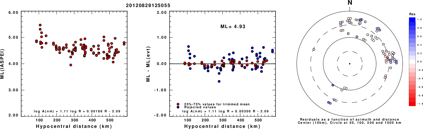
Left: ML computed using the IASPEI formula for Horizontal components. Center: ML residuals computed using a modified IASPEI formula that accounts for path specific attenuation; the values used for the trimmed mean are indicated. The ML relation used for each figure is given at the bottom of each plot.
Right: Residuals from new relation as a function of distance and azimuth.
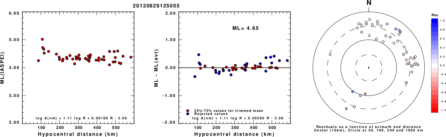
Left: ML computed using the IASPEI formula for Vertical components (research). Center: ML residuals computed using a modified IASPEI formula that accounts for path specific attenuation; the values used for the trimmed mean are indicated. The ML relation used for each figure is given at the bottom of each plot.
Right: Residuals from new relation as a function of distance and azimuth.
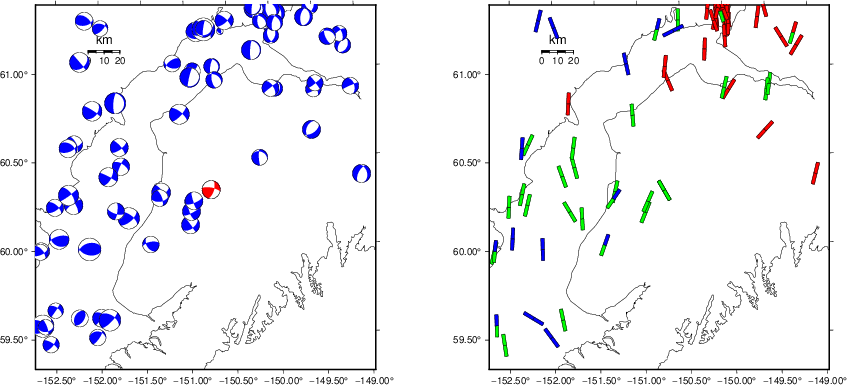
Context
The left panel of the next figure presents the focal mechanism for this earthquake (red) in the context of other nearby events (blue) in the SLU Moment Tensor Catalog. The right panel shows the inferred direction of maximum compressive stress and the type of faulting (green is strike-slip, red is normal, blue is thrust; oblique is shown by a combination of colors). Thus context plot is useful for assessing the appropriateness of the moment tensor of this event.
Waveform Inversion using wvfgrd96
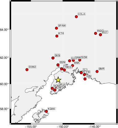
The focal mechanism was determined using broadband seismic waveforms. The location of the event (star) and the
stations used for (red) the waveform inversion are shown in the next figure.
|
|
Location of broadband stations used for waveform inversion
|
The program wvfgrd96 was used with good traces observed at short distance to determine the focal mechanism, depth and seismic moment. This technique requires a high quality signal and well determined velocity model for the Green's functions. To the extent that these are the quality data, this type of mechanism should be preferred over the radiation pattern technique which requires the separate step of defining the pressure and tension quadrants and the correct strike.
The observed and predicted traces are filtered using the following gsac commands:
hp c 0.02 n 3
lp c 0.06 n 3
The results of this grid search are as follow:
           DEPTH  STK   DIP  RAKE   MW    FIT
WVFGRD96    0.5    10    65   -25   3.66 0.1594
WVFGRD96    1.0    25    85     5   3.66 0.1721
WVFGRD96    2.0    25    75    15   3.79 0.2304
WVFGRD96    3.0    25    65    10   3.85 0.2540
WVFGRD96    4.0    20    65    -5   3.87 0.2769
WVFGRD96    5.0    20    65    -5   3.90 0.2979
WVFGRD96    6.0    20    65    -5   3.93 0.3152
WVFGRD96    7.0    20    70    -5   3.95 0.3303
WVFGRD96    8.0    20    65   -10   3.99 0.3433
WVFGRD96    9.0    20    65   -10   4.00 0.3531
WVFGRD96   10.0    20    65   -10   4.01 0.3605
WVFGRD96   11.0    20    70   -15   4.03 0.3671
WVFGRD96   12.0    20    70   -15   4.05 0.3726
WVFGRD96   13.0    20    70   -15   4.06 0.3768
WVFGRD96   14.0    20    70   -15   4.07 0.3800
WVFGRD96   15.0    20    70   -15   4.08 0.3832
WVFGRD96   16.0    15    70   -20   4.09 0.3869
WVFGRD96   17.0    15    70   -20   4.10 0.3901
WVFGRD96   18.0    15    70   -20   4.11 0.3933
WVFGRD96   19.0    15    70   -20   4.12 0.3967
WVFGRD96   20.0    15    70   -20   4.13 0.3999
WVFGRD96   21.0    15    70   -20   4.14 0.4025
WVFGRD96   22.0    15    70   -15   4.14 0.4049
WVFGRD96   23.0    15    70   -20   4.15 0.4072
WVFGRD96   24.0    15    70   -15   4.16 0.4099
WVFGRD96   25.0    15    70   -15   4.17 0.4122
WVFGRD96   26.0    15    70   -15   4.17 0.4142
WVFGRD96   27.0    15    70   -10   4.18 0.4159
WVFGRD96   28.0    15    70   -10   4.19 0.4174
WVFGRD96   29.0    15    70   -10   4.20 0.4191
WVFGRD96   30.0    15    70   -10   4.20 0.4205
WVFGRD96   31.0    15    70   -10   4.21 0.4215
WVFGRD96   32.0    15    70    -5   4.22 0.4220
WVFGRD96   33.0    15    70    -5   4.23 0.4222
WVFGRD96   34.0    15    70    -5   4.24 0.4221
WVFGRD96   35.0    15    70     0   4.25 0.4233
WVFGRD96   36.0    15    70     0   4.26 0.4248
WVFGRD96   37.0    15    70     0   4.27 0.4264
WVFGRD96   38.0    15    70     0   4.28 0.4276
WVFGRD96   39.0    15    70     0   4.29 0.4286
WVFGRD96   40.0    15    60     5   4.34 0.4301
WVFGRD96   41.0    15    60     5   4.35 0.4306
WVFGRD96   42.0    15    60     5   4.35 0.4310
WVFGRD96   43.0    15    65     5   4.36 0.4315
WVFGRD96   44.0    15    65     5   4.37 0.4321
WVFGRD96   45.0    15    65    10   4.38 0.4328
WVFGRD96   46.0    15    65    10   4.39 0.4335
WVFGRD96   47.0    20    65    15   4.40 0.4346
WVFGRD96   48.0    20    65    15   4.40 0.4363
WVFGRD96   49.0    20    65    20   4.42 0.4389
WVFGRD96   50.0    20    65    20   4.42 0.4423
WVFGRD96   51.0    20    65    20   4.43 0.4455
WVFGRD96   52.0    20    65    20   4.44 0.4484
WVFGRD96   53.0    20    65    20   4.44 0.4514
WVFGRD96   54.0    20    65    20   4.45 0.4546
WVFGRD96   55.0    20    65    20   4.46 0.4574
WVFGRD96   56.0    20    65    20   4.46 0.4599
WVFGRD96   57.0    20    65    20   4.47 0.4627
WVFGRD96   58.0    20    65    20   4.47 0.4656
WVFGRD96   59.0    20    65    20   4.48 0.4680
WVFGRD96   60.0    20    65    20   4.48 0.4695
WVFGRD96   61.0    20    65    20   4.49 0.4713
WVFGRD96   62.0    20    65    20   4.49 0.4737
WVFGRD96   63.0    20    65    20   4.50 0.4749
WVFGRD96   64.0    20    65    20   4.50 0.4761
WVFGRD96   65.0    20    65    20   4.50 0.4775
WVFGRD96   66.0    20    65    20   4.51 0.4784
WVFGRD96   67.0    20    65    20   4.51 0.4794
WVFGRD96   68.0    20    65    20   4.51 0.4795
WVFGRD96   69.0    20    65    20   4.52 0.4804
WVFGRD96   70.0    20    65    20   4.52 0.4809
WVFGRD96   71.0    20    65    20   4.52 0.4803
WVFGRD96   72.0    20    65    20   4.53 0.4811
WVFGRD96   73.0    20    65    20   4.53 0.4805
WVFGRD96   74.0    20    65    20   4.53 0.4802
WVFGRD96   75.0    20    65    20   4.54 0.4802
WVFGRD96   76.0    20    65    20   4.54 0.4786
WVFGRD96   77.0    20    65    20   4.54 0.4789
WVFGRD96   78.0    20    65    20   4.54 0.4777
WVFGRD96   79.0    20    65    20   4.55 0.4768
WVFGRD96   80.0    20    65    20   4.55 0.4758
WVFGRD96   81.0    20    65    20   4.55 0.4743
WVFGRD96   82.0    20    65    20   4.55 0.4735
WVFGRD96   83.0    20    65    20   4.56 0.4716
WVFGRD96   84.0    20    65    20   4.56 0.4708
WVFGRD96   85.0    20    65    20   4.56 0.4689
WVFGRD96   86.0    20    65    20   4.56 0.4676
WVFGRD96   87.0    20    65    20   4.56 0.4661
WVFGRD96   88.0    25    65    20   4.56 0.4643
WVFGRD96   89.0    25    65    20   4.57 0.4632
WVFGRD96   90.0    25    65    20   4.57 0.4616
WVFGRD96   91.0    25    65    20   4.57 0.4603
WVFGRD96   92.0    25    65    20   4.57 0.4587
WVFGRD96   93.0    25    65    20   4.57 0.4571
WVFGRD96   94.0    25    70    20   4.58 0.4556
WVFGRD96   95.0    25    70    20   4.58 0.4543
WVFGRD96   96.0    25    70    20   4.58 0.4531
WVFGRD96   97.0    25    70    20   4.58 0.4516
WVFGRD96   98.0    25    70    20   4.58 0.4505
WVFGRD96   99.0    25    70    20   4.59 0.4490
The best solution is
WVFGRD96 72.0 20 65 20 4.53 0.4811
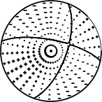
The mechanism corresponding to the best fit is
|
|
Figure 1. Waveform inversion focal mechanism
|
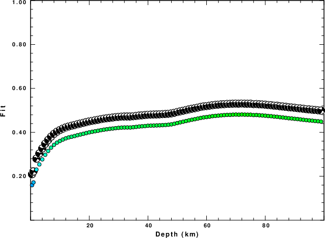
The best fit as a function of depth is given in the following figure:
|
|
Figure 2. Depth sensitivity for waveform mechanism
|
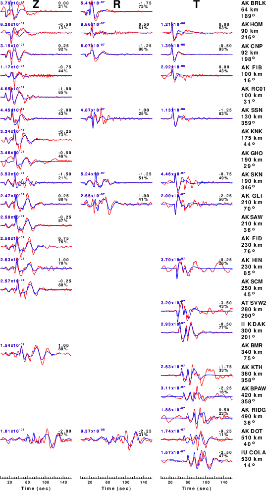
The comparison of the observed and predicted waveforms is given in the next figure. The red traces are the observed and the blue are the predicted.
Each observed-predicted component is plotted to the same scale and peak amplitudes are indicated by the numbers to the left of each trace. A pair of numbers is given in black at the right of each predicted traces. The upper number it the time shift required for maximum correlation between the observed and predicted traces. This time shift is required because the synthetics are not computed at exactly the same distance as the observed, the velocity model used in the predictions may not be perfect and the epicentral parameters may be be off.
A positive time shift indicates that the prediction is too fast and should be delayed to match the observed trace (shift to the right in this figure). A negative value indicates that the prediction is too slow. The lower number gives the percentage of variance reduction to characterize the individual goodness of fit (100% indicates a perfect fit).
The bandpass filter used in the processing and for the display was
hp c 0.02 n 3
lp c 0.06 n 3
|
|
Figure 3. Waveform comparison for selected depth. Red: observed; Blue - predicted. The time shift with respect to the model prediction is indicated. The percent of fit is also indicated. The time scale is relative to the first trace sample.
|
|
|
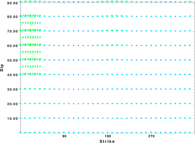
Focal mechanism sensitivity at the preferred depth. The red color indicates a very good fit to the waveforms.
Each solution is plotted as a vector at a given value of strike and dip with the angle of the vector representing the rake angle, measured, with respect to the upward vertical (N) in the figure.
|
A check on the assumed source location is possible by looking at the time shifts between the observed and predicted traces. The time shifts for waveform matching arise for several reasons:
- The origin time and epicentral distance are incorrect
- The velocity model used for the inversion is incorrect
- The velocity model used to define the P-arrival time is not the
same as the velocity model used for the waveform inversion
(assuming that the initial trace alignment is based on the
P arrival time)
Assuming only a mislocation, the time shifts are fit to a functional form:
Time_shift = A + B cos Azimuth + C Sin Azimuth
The time shifts for this inversion lead to the next figure:
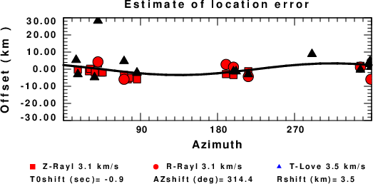
The derived shift in origin time and epicentral coordinates are given at the bottom of the figure.
Velocity Model
The WUS.model used for the waveform synthetic seismograms and for the surface wave eigenfunctions and dispersion is as follows
(The format is in the model96 format of Computer Programs in Seismology).
MODEL.01
Model after     8 iterations
ISOTROPIC
KGS
FLAT EARTH
1-D
CONSTANT VELOCITY
LINE08
LINE09
LINE10
LINE11
      H(KM)   VP(KM/S)   VS(KM/S) RHO(GM/CC)         QP         QS       ETAP       ETAS      FREFP      FREFS
     1.9000     3.4065     2.0089     2.2150  0.302E-02  0.679E-02   0.00       0.00       1.00       1.00
     6.1000     5.5445     3.2953     2.6089  0.349E-02  0.784E-02   0.00       0.00       1.00       1.00
    13.0000     6.2708     3.7396     2.7812  0.212E-02  0.476E-02   0.00       0.00       1.00       1.00
    19.0000     6.4075     3.7680     2.8223  0.111E-02  0.249E-02   0.00       0.00       1.00       1.00
     0.0000     7.9000     4.6200     3.2760  0.164E-10  0.370E-10   0.00       0.00       1.00       1.00
Last Changed Fri Apr 26 10:40:06 PM CDT 2024