Location
Location ANSS
The ANSS event ID is ak0128tllrpw and the event page is at
https://earthquake.usgs.gov/earthquakes/eventpage/ak0128tllrpw/executive.
2012/07/10 04:06:54 63.439 -149.394 104.0 4.2 Alaska
Focal Mechanism
 USGS/SLU Moment Tensor Solution
 ENS  2012/07/10 04:06:54:0  63.44 -149.39 104.0 4.2 Alaska

 Stations used:
   AK.BPAW AK.BWN AK.CCB AK.GHO AK.GLM AK.KNK AK.KTH AK.MDM
   AK.MLY AK.NEA AK.PAX AK.PPLA AK.SAW AK.SCM AK.TRF AK.WRH

 Filtering commands used:
   hp c 0.02 n 3
   lp c 0.10 n 3

 Best Fitting Double Couple
  Mo = 3.31e+22 dyne-cm
  Mw = 4.28
  Z  = 122 km
  Plane   Strike  Dip  Rake
   NP1      324    58   138
   NP2       80    55    40
  Principal Axes:
   Axis    Value   Plunge  Azimuth
    T   3.31e+22     51     290
    N   0.00e+00     39     114
    P  -3.31e+22      2      23

 Moment Tensor: (dyne-cm)
    Component   Value
       Mxx    -2.65e+22
       Mxy    -1.61e+22
       Mxz     4.64e+21
       Myy     6.50e+21
       Myz    -1.56e+22
       Mzz     2.00e+22


                     ------------ P
                 ----------------   ---
              #######---------------------
             ############------------------
           #################-----------------
          ####################----------------
         #######################---------------
        #########################---------------
        #########   ###############-------------
       ########## T ################------------#
       ##########   #################----------##
       ###############################-------####
       ################################----######
        -##############################--#######
        ----#########################---########
         -------###############---------#######
          -------------------------------#####
           ------------------------------####
             ----------------------------##
              --------------------------##
                 ----------------------
                     --------------


 Global CMT Convention Moment Tensor:
      R          T          P
  2.00e+22   4.64e+21   1.56e+22
  4.64e+21  -2.65e+22   1.61e+22
  1.56e+22   1.61e+22   6.50e+21


Details of the solution is found at

http://www.eas.slu.edu/eqc/eqc_mt/MECH.NA/20120710040654/index.html
|
Preferred Solution
The preferred solution from an analysis of the surface-wave spectral amplitude radiation pattern, waveform inversion or first motion observations is
      STK = 80
      DIP = 55
     RAKE = 40
       MW = 4.28
       HS = 122.0
The NDK file is 20120710040654.ndk
The waveform inversion is preferred.
Magnitudes
Given the availability of digital waveforms for determination of the moment tensor, this section documents the added processing leading to mLg, if appropriate to the region, and ML by application of the respective IASPEI formulae. As a research study, the linear distance term of the IASPEI formula
for ML is adjusted to remove a linear distance trend in residuals to give a regionally defined ML. The defined ML uses horizontal component recordings, but the same procedure is applied to the vertical components since there may be some interest in vertical component ground motions. Residual plots versus distance may indicate interesting features of ground motion scaling in some distance ranges. A residual plot of the regionalized magnitude is given as a function of distance and azimuth, since data sets may transcend different wave propagation provinces.
ML Magnitude
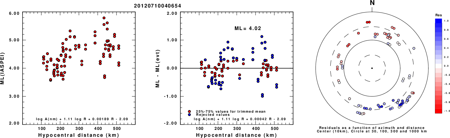
Left: ML computed using the IASPEI formula for Horizontal components. Center: ML residuals computed using a modified IASPEI formula that accounts for path specific attenuation; the values used for the trimmed mean are indicated. The ML relation used for each figure is given at the bottom of each plot.
Right: Residuals from new relation as a function of distance and azimuth.
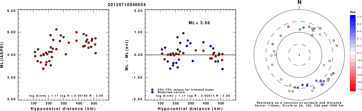
Left: ML computed using the IASPEI formula for Vertical components (research). Center: ML residuals computed using a modified IASPEI formula that accounts for path specific attenuation; the values used for the trimmed mean are indicated. The ML relation used for each figure is given at the bottom of each plot.
Right: Residuals from new relation as a function of distance and azimuth.
Context
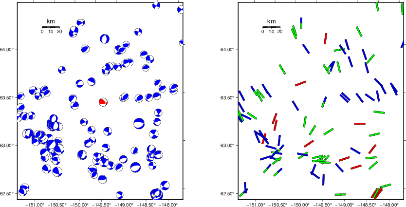
The left panel of the next figure presents the focal mechanism for this earthquake (red) in the context of other nearby events (blue) in the SLU Moment Tensor Catalog. The right panel shows the inferred direction of maximum compressive stress and the type of faulting (green is strike-slip, red is normal, blue is thrust; oblique is shown by a combination of colors). Thus context plot is useful for assessing the appropriateness of the moment tensor of this event.
Waveform Inversion using wvfgrd96
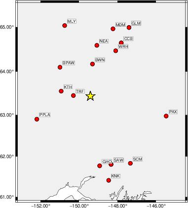
The focal mechanism was determined using broadband seismic waveforms. The location of the event (star) and the
stations used for (red) the waveform inversion are shown in the next figure.
|
|
Location of broadband stations used for waveform inversion
|
The program wvfgrd96 was used with good traces observed at short distance to determine the focal mechanism, depth and seismic moment. This technique requires a high quality signal and well determined velocity model for the Green's functions. To the extent that these are the quality data, this type of mechanism should be preferred over the radiation pattern technique which requires the separate step of defining the pressure and tension quadrants and the correct strike.
The observed and predicted traces are filtered using the following gsac commands:
hp c 0.02 n 3
lp c 0.10 n 3
The results of this grid search are as follow:
           DEPTH  STK   DIP  RAKE   MW    FIT
WVFGRD96    0.5   110    50   -90   3.15 0.2028
WVFGRD96    1.0   310    45   -55   3.17 0.1923
WVFGRD96    2.0   295    40   -80   3.35 0.2756
WVFGRD96    3.0   295    40   -75   3.41 0.2676
WVFGRD96    4.0   335    60   -20   3.37 0.2360
WVFGRD96    5.0   170    50    10   3.41 0.2509
WVFGRD96    6.0   170    55    10   3.44 0.2703
WVFGRD96    7.0   165    50     5   3.44 0.2881
WVFGRD96    8.0   165    45    10   3.50 0.3005
WVFGRD96    9.0   165    50    10   3.53 0.3100
WVFGRD96   10.0   180    60    20   3.59 0.3185
WVFGRD96   11.0   180    65    20   3.63 0.3261
WVFGRD96   12.0   180    65    20   3.65 0.3329
WVFGRD96   13.0   180    65    20   3.66 0.3338
WVFGRD96   14.0   180    65    20   3.68 0.3361
WVFGRD96   15.0   180    65    20   3.69 0.3362
WVFGRD96   16.0   180    65    20   3.71 0.3315
WVFGRD96   17.0   185    65    20   3.73 0.3303
WVFGRD96   18.0   185    65    20   3.74 0.3259
WVFGRD96   19.0   185    65    20   3.76 0.3241
WVFGRD96   20.0   185    65    20   3.77 0.3211
WVFGRD96   21.0   190    65    15   3.79 0.3083
WVFGRD96   22.0   190    65    15   3.81 0.3042
WVFGRD96   23.0   190    65    15   3.81 0.2951
WVFGRD96   24.0   190    70    15   3.83 0.2748
WVFGRD96   25.0   190    70    15   3.84 0.2659
WVFGRD96   26.0   240    45    30   3.70 0.2595
WVFGRD96   27.0   240    50    25   3.71 0.2610
WVFGRD96   28.0   240    50    25   3.72 0.2627
WVFGRD96   29.0   240    50    25   3.73 0.2601
WVFGRD96   30.0     0    60   -25   3.83 0.2657
WVFGRD96   31.0     0    60   -25   3.84 0.2746
WVFGRD96   32.0     0    60   -25   3.86 0.2818
WVFGRD96   33.0     0    60   -25   3.87 0.2872
WVFGRD96   34.0     0    60   -20   3.88 0.2929
WVFGRD96   35.0     0    65   -20   3.92 0.2991
WVFGRD96   36.0     5    70   -15   3.95 0.3068
WVFGRD96   37.0     5    70   -10   3.97 0.3166
WVFGRD96   38.0     5    75    -5   4.01 0.3277
WVFGRD96   39.0     5    75    -5   4.03 0.3412
WVFGRD96   40.0     5    70   -10   4.08 0.3573
WVFGRD96   41.0     5    70    -5   4.10 0.3644
WVFGRD96   42.0     5    70    -5   4.11 0.3702
WVFGRD96   43.0     5    65    -5   4.11 0.3761
WVFGRD96   44.0     5    65    -5   4.12 0.3827
WVFGRD96   45.0     5    65    -5   4.13 0.3883
WVFGRD96   46.0     5    65    -5   4.14 0.3934
WVFGRD96   47.0     5    65    -5   4.15 0.3970
WVFGRD96   48.0     5    65    -5   4.16 0.3995
WVFGRD96   49.0     5    60    -5   4.14 0.4017
WVFGRD96   50.0    10    65    15   4.16 0.4059
WVFGRD96   51.0    10    65    15   4.17 0.4103
WVFGRD96   52.0    15    60    25   4.15 0.4165
WVFGRD96   53.0    15    60    25   4.15 0.4216
WVFGRD96   54.0    15    60    25   4.16 0.4257
WVFGRD96   55.0    15    65    25   4.19 0.4286
WVFGRD96   56.0    80    85   -30   4.15 0.4346
WVFGRD96   57.0   260    90    30   4.14 0.4373
WVFGRD96   58.0    80    85   -30   4.15 0.4484
WVFGRD96   59.0    80    85   -30   4.16 0.4541
WVFGRD96   60.0   260    90    30   4.15 0.4569
WVFGRD96   61.0    80    85   -30   4.16 0.4635
WVFGRD96   62.0    80    45    45   4.13 0.4787
WVFGRD96   63.0    80    45    45   4.13 0.4917
WVFGRD96   64.0    80    45    45   4.13 0.5028
WVFGRD96   65.0    80    45    40   4.15 0.5143
WVFGRD96   66.0    80    50    40   4.16 0.5247
WVFGRD96   67.0    80    50    40   4.16 0.5355
WVFGRD96   68.0    80    50    40   4.17 0.5455
WVFGRD96   69.0    80    50    40   4.17 0.5545
WVFGRD96   70.0    75    50    35   4.17 0.5624
WVFGRD96   71.0    75    50    35   4.17 0.5703
WVFGRD96   72.0    80    50    40   4.18 0.5769
WVFGRD96   73.0    80    50    40   4.18 0.5855
WVFGRD96   74.0    75    50    35   4.18 0.5918
WVFGRD96   75.0    75    50    35   4.18 0.5982
WVFGRD96   76.0    75    50    35   4.18 0.6048
WVFGRD96   77.0    75    50    35   4.18 0.6104
WVFGRD96   78.0    75    50    35   4.19 0.6170
WVFGRD96   79.0    75    50    35   4.19 0.6215
WVFGRD96   80.0    75    50    35   4.19 0.6276
WVFGRD96   81.0    75    50    35   4.20 0.6323
WVFGRD96   82.0    75    50    35   4.20 0.6388
WVFGRD96   83.0    75    50    35   4.20 0.6414
WVFGRD96   84.0    75    50    35   4.20 0.6473
WVFGRD96   85.0    75    50    35   4.21 0.6517
WVFGRD96   86.0    75    50    35   4.21 0.6564
WVFGRD96   87.0    75    50    40   4.20 0.6591
WVFGRD96   88.0    75    50    40   4.20 0.6657
WVFGRD96   89.0    75    50    40   4.21 0.6697
WVFGRD96   90.0    75    50    40   4.21 0.6734
WVFGRD96   91.0    75    50    40   4.21 0.6784
WVFGRD96   92.0    75    50    40   4.21 0.6816
WVFGRD96   93.0    75    50    40   4.22 0.6854
WVFGRD96   94.0    75    50    40   4.22 0.6889
WVFGRD96   95.0    75    50    40   4.22 0.6924
WVFGRD96   96.0    75    50    40   4.22 0.6945
WVFGRD96   97.0    75    50    40   4.23 0.6997
WVFGRD96   98.0    75    50    40   4.23 0.6995
WVFGRD96   99.0    75    50    40   4.23 0.7037
WVFGRD96  100.0    75    50    40   4.23 0.7063
WVFGRD96  101.0    75    50    40   4.23 0.7071
WVFGRD96  102.0    75    50    40   4.24 0.7103
WVFGRD96  103.0    75    50    40   4.24 0.7112
WVFGRD96  104.0    75    50    40   4.24 0.7131
WVFGRD96  105.0    75    50    40   4.24 0.7134
WVFGRD96  106.0    75    50    40   4.24 0.7161
WVFGRD96  107.0    75    50    40   4.24 0.7158
WVFGRD96  108.0    80    55    40   4.26 0.7188
WVFGRD96  109.0    80    55    40   4.26 0.7196
WVFGRD96  110.0    80    55    40   4.26 0.7201
WVFGRD96  111.0    80    55    40   4.26 0.7223
WVFGRD96  112.0    80    55    40   4.26 0.7219
WVFGRD96  113.0    80    55    40   4.27 0.7227
WVFGRD96  114.0    80    55    40   4.27 0.7242
WVFGRD96  115.0    80    55    40   4.27 0.7236
WVFGRD96  116.0    80    55    40   4.27 0.7248
WVFGRD96  117.0    80    55    40   4.27 0.7259
WVFGRD96  118.0    80    55    40   4.27 0.7243
WVFGRD96  119.0    80    55    40   4.27 0.7264
WVFGRD96  120.0    80    55    40   4.27 0.7266
WVFGRD96  121.0    80    55    40   4.27 0.7257
WVFGRD96  122.0    80    55    40   4.28 0.7272
WVFGRD96  123.0    80    55    40   4.28 0.7255
WVFGRD96  124.0    80    55    40   4.28 0.7266
WVFGRD96  125.0    80    55    40   4.28 0.7264
WVFGRD96  126.0    80    55    40   4.28 0.7269
WVFGRD96  127.0    80    55    40   4.28 0.7256
WVFGRD96  128.0    80    55    40   4.28 0.7256
WVFGRD96  129.0    80    55    40   4.28 0.7258
The best solution is
WVFGRD96 122.0 80 55 40 4.28 0.7272
The mechanism corresponding to the best fit is
|
|
Figure 1. Waveform inversion focal mechanism
|
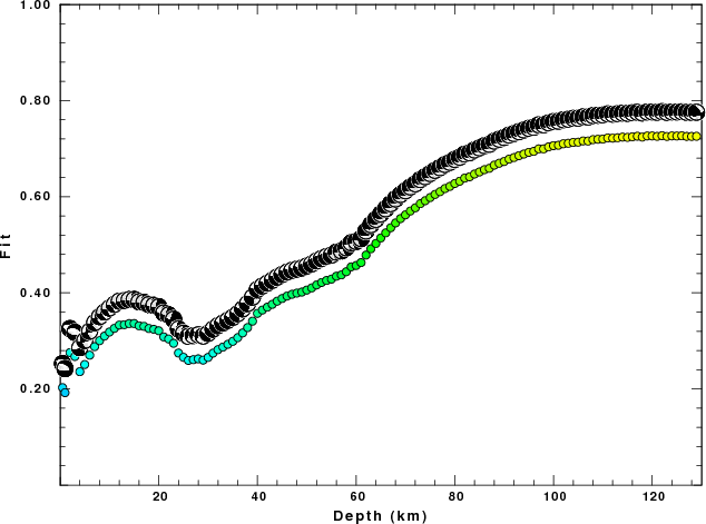
The best fit as a function of depth is given in the following figure:
|
|
Figure 2. Depth sensitivity for waveform mechanism
|
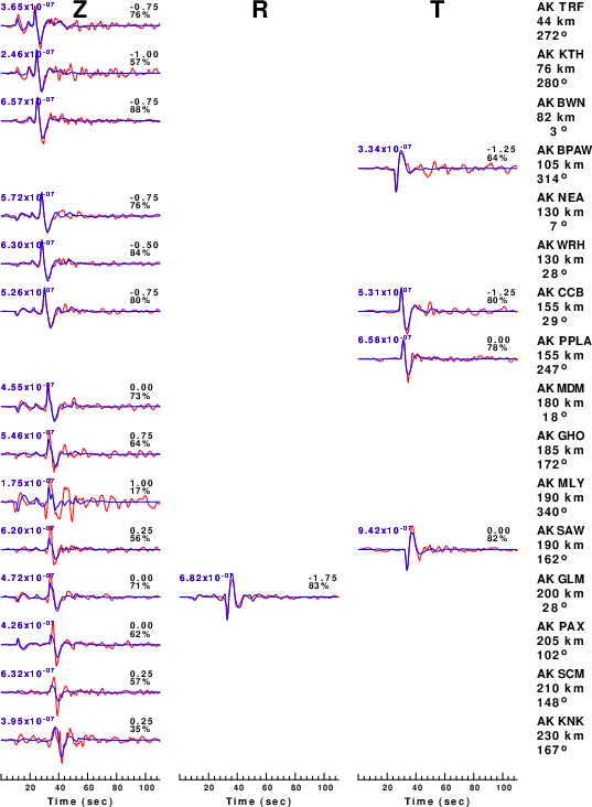
The comparison of the observed and predicted waveforms is given in the next figure. The red traces are the observed and the blue are the predicted.
Each observed-predicted component is plotted to the same scale and peak amplitudes are indicated by the numbers to the left of each trace. A pair of numbers is given in black at the right of each predicted traces. The upper number it the time shift required for maximum correlation between the observed and predicted traces. This time shift is required because the synthetics are not computed at exactly the same distance as the observed, the velocity model used in the predictions may not be perfect and the epicentral parameters may be be off.
A positive time shift indicates that the prediction is too fast and should be delayed to match the observed trace (shift to the right in this figure). A negative value indicates that the prediction is too slow. The lower number gives the percentage of variance reduction to characterize the individual goodness of fit (100% indicates a perfect fit).
The bandpass filter used in the processing and for the display was
hp c 0.02 n 3
lp c 0.10 n 3
|
|
Figure 3. Waveform comparison for selected depth. Red: observed; Blue - predicted. The time shift with respect to the model prediction is indicated. The percent of fit is also indicated. The time scale is relative to the first trace sample.
|
|
|
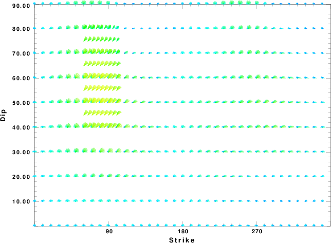
Focal mechanism sensitivity at the preferred depth. The red color indicates a very good fit to the waveforms.
Each solution is plotted as a vector at a given value of strike and dip with the angle of the vector representing the rake angle, measured, with respect to the upward vertical (N) in the figure.
|
A check on the assumed source location is possible by looking at the time shifts between the observed and predicted traces. The time shifts for waveform matching arise for several reasons:
- The origin time and epicentral distance are incorrect
- The velocity model used for the inversion is incorrect
- The velocity model used to define the P-arrival time is not the
same as the velocity model used for the waveform inversion
(assuming that the initial trace alignment is based on the
P arrival time)
Assuming only a mislocation, the time shifts are fit to a functional form:
Time_shift = A + B cos Azimuth + C Sin Azimuth
The time shifts for this inversion lead to the next figure:
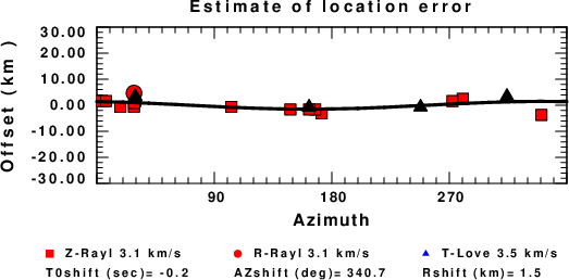
The derived shift in origin time and epicentral coordinates are given at the bottom of the figure.
Velocity Model
The WUS.model used for the waveform synthetic seismograms and for the surface wave eigenfunctions and dispersion is as follows
(The format is in the model96 format of Computer Programs in Seismology).
MODEL.01
Model after     8 iterations
ISOTROPIC
KGS
FLAT EARTH
1-D
CONSTANT VELOCITY
LINE08
LINE09
LINE10
LINE11
      H(KM)   VP(KM/S)   VS(KM/S) RHO(GM/CC)         QP         QS       ETAP       ETAS      FREFP      FREFS
     1.9000     3.4065     2.0089     2.2150  0.302E-02  0.679E-02   0.00       0.00       1.00       1.00
     6.1000     5.5445     3.2953     2.6089  0.349E-02  0.784E-02   0.00       0.00       1.00       1.00
    13.0000     6.2708     3.7396     2.7812  0.212E-02  0.476E-02   0.00       0.00       1.00       1.00
    19.0000     6.4075     3.7680     2.8223  0.111E-02  0.249E-02   0.00       0.00       1.00       1.00
     0.0000     7.9000     4.6200     3.2760  0.164E-10  0.370E-10   0.00       0.00       1.00       1.00
Last Changed Fri Apr 26 09:51:35 PM CDT 2024