Location
Location ANSS
The ANSS event ID is ak0127cwv72m and the event page is at
https://earthquake.usgs.gov/earthquakes/eventpage/ak0127cwv72m/executive.
2012/06/08 18:27:36 62.226 -147.875 40.4 4.2 Alaska
Focal Mechanism
 USGS/SLU Moment Tensor Solution
 ENS  2012/06/08 18:27:36:0  62.23 -147.88  40.4 4.2 Alaska

 Stations used:
   AK.BAL AK.BMR AK.BWN AK.CCB AK.COLD AK.CRQ AK.CTG AK.DHY
   AK.DIV AK.FYU AK.GHO AK.GLM AK.HDA AK.KLU AK.KNK AK.KTH
   AK.MCK AK.MDM AK.MLY AK.PAX AK.PPD AK.PPLA AK.RAG AK.RIDG
   AK.RND AK.SAW AK.SCM AK.SCRK AK.TGL AK.TRF AK.WRH AT.PMR
   CN.DAWY IU.COLA US.EGAK

 Filtering commands used:
   hp c 0.02 n 3
   lp c 0.06 n 3

 Best Fitting Double Couple
  Mo = 2.69e+22 dyne-cm
  Mw = 4.22
  Z  = 51 km
  Plane   Strike  Dip  Rake
   NP1      255    60   -40
   NP2        8    56   -143
  Principal Axes:
   Axis    Value   Plunge  Azimuth
    T   2.69e+22      2     312
    N   0.00e+00     42      44
    P  -2.69e+22     48     220

 Moment Tensor: (dyne-cm)
    Component   Value
       Mxx     5.05e+21
       Mxy    -1.92e+22
       Mxz     1.10e+22
       Myy     9.93e+21
       Myz     7.72e+21
       Mzz    -1.50e+22


                     ###########---
                 ################------
               ###################--------
             T ####################--------
           #   #####################---------
          ##########################----------
         ######################-----####-------
        ###############--------------#########--
        ###########------------------###########
       #########---------------------############
       ######------------------------############
       ####-------------------------#############
       ###--------------------------#############
        ----------------------------############
        ------------   ------------#############
         ----------- P ------------############
          ----------   -----------############
           ----------------------############
             -------------------###########
              -----------------###########
                 ------------##########
                     ------########


 Global CMT Convention Moment Tensor:
      R          T          P
 -1.50e+22   1.10e+22  -7.72e+21
  1.10e+22   5.05e+21   1.92e+22
 -7.72e+21   1.92e+22   9.93e+21


Details of the solution is found at

http://www.eas.slu.edu/eqc/eqc_mt/MECH.NA/20120608182736/index.html
|
Preferred Solution
The preferred solution from an analysis of the surface-wave spectral amplitude radiation pattern, waveform inversion or first motion observations is
      STK = 255
      DIP = 60
     RAKE = -40
       MW = 4.22
       HS = 51.0
The NDK file is 20120608182736.ndk
The waveform inversion is preferred.
Magnitudes
Given the availability of digital waveforms for determination of the moment tensor, this section documents the added processing leading to mLg, if appropriate to the region, and ML by application of the respective IASPEI formulae. As a research study, the linear distance term of the IASPEI formula
for ML is adjusted to remove a linear distance trend in residuals to give a regionally defined ML. The defined ML uses horizontal component recordings, but the same procedure is applied to the vertical components since there may be some interest in vertical component ground motions. Residual plots versus distance may indicate interesting features of ground motion scaling in some distance ranges. A residual plot of the regionalized magnitude is given as a function of distance and azimuth, since data sets may transcend different wave propagation provinces.
ML Magnitude
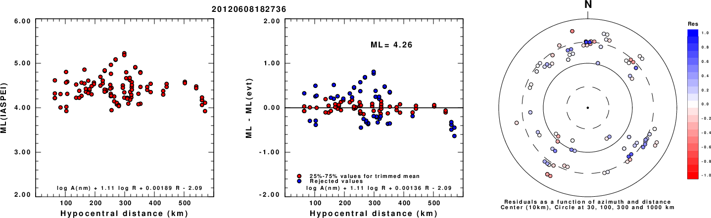
Left: ML computed using the IASPEI formula for Horizontal components. Center: ML residuals computed using a modified IASPEI formula that accounts for path specific attenuation; the values used for the trimmed mean are indicated. The ML relation used for each figure is given at the bottom of each plot.
Right: Residuals from new relation as a function of distance and azimuth.
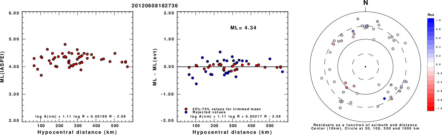
Left: ML computed using the IASPEI formula for Vertical components (research). Center: ML residuals computed using a modified IASPEI formula that accounts for path specific attenuation; the values used for the trimmed mean are indicated. The ML relation used for each figure is given at the bottom of each plot.
Right: Residuals from new relation as a function of distance and azimuth.
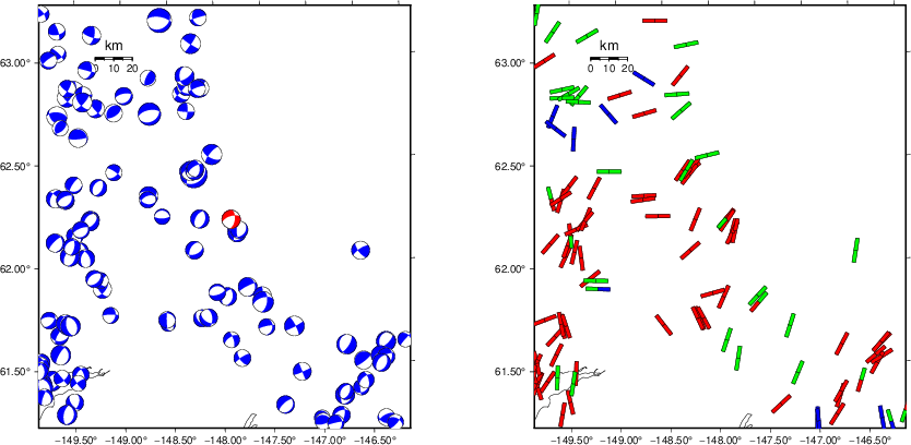
Context
The left panel of the next figure presents the focal mechanism for this earthquake (red) in the context of other nearby events (blue) in the SLU Moment Tensor Catalog. The right panel shows the inferred direction of maximum compressive stress and the type of faulting (green is strike-slip, red is normal, blue is thrust; oblique is shown by a combination of colors). Thus context plot is useful for assessing the appropriateness of the moment tensor of this event.
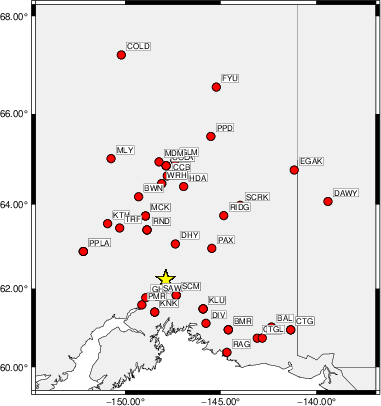
Waveform Inversion using wvfgrd96
The focal mechanism was determined using broadband seismic waveforms. The location of the event (star) and the
stations used for (red) the waveform inversion are shown in the next figure.
|
|
Location of broadband stations used for waveform inversion
|
The program wvfgrd96 was used with good traces observed at short distance to determine the focal mechanism, depth and seismic moment. This technique requires a high quality signal and well determined velocity model for the Green's functions. To the extent that these are the quality data, this type of mechanism should be preferred over the radiation pattern technique which requires the separate step of defining the pressure and tension quadrants and the correct strike.
The observed and predicted traces are filtered using the following gsac commands:
hp c 0.02 n 3
lp c 0.06 n 3
The results of this grid search are as follow:
           DEPTH  STK   DIP  RAKE   MW    FIT
WVFGRD96    0.5   230    45    95   3.41 0.2288
WVFGRD96    1.0   230    45    90   3.45 0.2389
WVFGRD96    2.0    50    45    95   3.56 0.3002
WVFGRD96    3.0   225    45    85   3.63 0.3090
WVFGRD96    4.0     0    75    15   3.58 0.2970
WVFGRD96    5.0     0    80    15   3.60 0.2871
WVFGRD96    6.0    90    80   -10   3.62 0.2893
WVFGRD96    7.0   275    70    30   3.66 0.3032
WVFGRD96    8.0   275    70    35   3.71 0.3184
WVFGRD96    9.0   275    70    35   3.72 0.3263
WVFGRD96   10.0   275    70    35   3.73 0.3304
WVFGRD96   11.0   275    70    35   3.74 0.3325
WVFGRD96   12.0   275    70    35   3.75 0.3333
WVFGRD96   13.0   280    65    35   3.76 0.3344
WVFGRD96   14.0     5    90    60   3.77 0.3392
WVFGRD96   15.0   105    60    50   3.75 0.3489
WVFGRD96   16.0    80    75   -45   3.75 0.3603
WVFGRD96   17.0    80    75   -45   3.76 0.3751
WVFGRD96   18.0    80    75   -45   3.77 0.3882
WVFGRD96   19.0    80    75   -45   3.78 0.4001
WVFGRD96   20.0    80    70   -45   3.79 0.4109
WVFGRD96   21.0    80    70   -45   3.81 0.4228
WVFGRD96   22.0    80    70   -40   3.83 0.4333
WVFGRD96   23.0    80    70   -40   3.84 0.4433
WVFGRD96   24.0    80    70   -40   3.85 0.4520
WVFGRD96   25.0   260    45   -30   3.88 0.4638
WVFGRD96   26.0   260    50   -30   3.89 0.4748
WVFGRD96   27.0   260    50   -30   3.90 0.4858
WVFGRD96   28.0   260    50   -30   3.92 0.4957
WVFGRD96   29.0   260    50   -30   3.93 0.5043
WVFGRD96   30.0   260    50   -30   3.94 0.5120
WVFGRD96   31.0   260    55   -30   3.95 0.5197
WVFGRD96   32.0   260    55   -25   3.97 0.5278
WVFGRD96   33.0   260    60   -30   3.97 0.5384
WVFGRD96   34.0   260    60   -30   3.98 0.5485
WVFGRD96   35.0   260    60   -30   3.99 0.5578
WVFGRD96   36.0   260    60   -30   4.00 0.5661
WVFGRD96   37.0   260    60   -30   4.02 0.5729
WVFGRD96   38.0   260    60   -30   4.03 0.5781
WVFGRD96   39.0   260    60   -30   4.04 0.5797
WVFGRD96   40.0   255    55   -35   4.14 0.6033
WVFGRD96   41.0   255    55   -35   4.15 0.6136
WVFGRD96   42.0   255    60   -35   4.15 0.6225
WVFGRD96   43.0   255    60   -40   4.16 0.6310
WVFGRD96   44.0   255    60   -40   4.16 0.6382
WVFGRD96   45.0   255    60   -40   4.17 0.6438
WVFGRD96   46.0   255    60   -40   4.18 0.6488
WVFGRD96   47.0   255    60   -40   4.19 0.6521
WVFGRD96   48.0   255    60   -40   4.20 0.6545
WVFGRD96   49.0   255    60   -40   4.20 0.6554
WVFGRD96   50.0   255    60   -40   4.21 0.6557
WVFGRD96   51.0   255    60   -40   4.22 0.6559
WVFGRD96   52.0   255    60   -40   4.22 0.6545
WVFGRD96   53.0   255    60   -40   4.23 0.6525
WVFGRD96   54.0   255    60   -35   4.24 0.6493
WVFGRD96   55.0   255    65   -35   4.24 0.6457
WVFGRD96   56.0   255    65   -35   4.24 0.6424
WVFGRD96   57.0   255    65   -35   4.25 0.6389
WVFGRD96   58.0   255    65   -35   4.25 0.6341
WVFGRD96   59.0   255    65   -35   4.26 0.6287
WVFGRD96   60.0   255    65   -35   4.26 0.6227
WVFGRD96   61.0   255    65   -35   4.26 0.6161
WVFGRD96   62.0   255    65   -35   4.26 0.6082
WVFGRD96   63.0   255    65   -35   4.27 0.6014
WVFGRD96   64.0   255    65   -35   4.27 0.5930
WVFGRD96   65.0   255    65   -35   4.27 0.5848
WVFGRD96   66.0   260    70   -30   4.26 0.5777
WVFGRD96   67.0   260    70   -30   4.27 0.5704
WVFGRD96   68.0   260    70   -30   4.27 0.5629
WVFGRD96   69.0   260    70   -30   4.27 0.5552
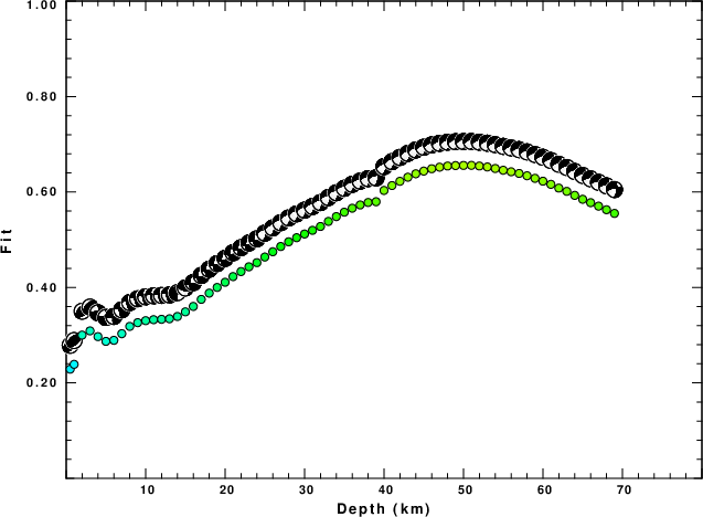
The best solution is
WVFGRD96 51.0 255 60 -40 4.22 0.6559
The mechanism corresponding to the best fit is
|
|
Figure 1. Waveform inversion focal mechanism
|
The best fit as a function of depth is given in the following figure:
|
|
Figure 2. Depth sensitivity for waveform mechanism
|
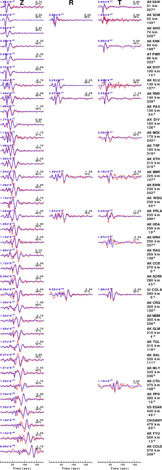
The comparison of the observed and predicted waveforms is given in the next figure. The red traces are the observed and the blue are the predicted.
Each observed-predicted component is plotted to the same scale and peak amplitudes are indicated by the numbers to the left of each trace. A pair of numbers is given in black at the right of each predicted traces. The upper number it the time shift required for maximum correlation between the observed and predicted traces. This time shift is required because the synthetics are not computed at exactly the same distance as the observed, the velocity model used in the predictions may not be perfect and the epicentral parameters may be be off.
A positive time shift indicates that the prediction is too fast and should be delayed to match the observed trace (shift to the right in this figure). A negative value indicates that the prediction is too slow. The lower number gives the percentage of variance reduction to characterize the individual goodness of fit (100% indicates a perfect fit).
The bandpass filter used in the processing and for the display was
hp c 0.02 n 3
lp c 0.06 n 3
|
|
Figure 3. Waveform comparison for selected depth. Red: observed; Blue - predicted. The time shift with respect to the model prediction is indicated. The percent of fit is also indicated. The time scale is relative to the first trace sample.
|
|
|
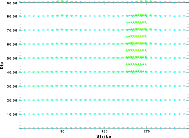
Focal mechanism sensitivity at the preferred depth. The red color indicates a very good fit to the waveforms.
Each solution is plotted as a vector at a given value of strike and dip with the angle of the vector representing the rake angle, measured, with respect to the upward vertical (N) in the figure.
|
A check on the assumed source location is possible by looking at the time shifts between the observed and predicted traces. The time shifts for waveform matching arise for several reasons:
- The origin time and epicentral distance are incorrect
- The velocity model used for the inversion is incorrect
- The velocity model used to define the P-arrival time is not the
same as the velocity model used for the waveform inversion
(assuming that the initial trace alignment is based on the
P arrival time)
Assuming only a mislocation, the time shifts are fit to a functional form:
Time_shift = A + B cos Azimuth + C Sin Azimuth
The time shifts for this inversion lead to the next figure:
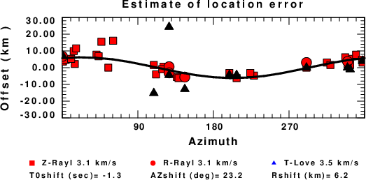
The derived shift in origin time and epicentral coordinates are given at the bottom of the figure.
Velocity Model
The WUS.model used for the waveform synthetic seismograms and for the surface wave eigenfunctions and dispersion is as follows
(The format is in the model96 format of Computer Programs in Seismology).
MODEL.01
Model after     8 iterations
ISOTROPIC
KGS
FLAT EARTH
1-D
CONSTANT VELOCITY
LINE08
LINE09
LINE10
LINE11
      H(KM)   VP(KM/S)   VS(KM/S) RHO(GM/CC)         QP         QS       ETAP       ETAS      FREFP      FREFS
     1.9000     3.4065     2.0089     2.2150  0.302E-02  0.679E-02   0.00       0.00       1.00       1.00
     6.1000     5.5445     3.2953     2.6089  0.349E-02  0.784E-02   0.00       0.00       1.00       1.00
    13.0000     6.2708     3.7396     2.7812  0.212E-02  0.476E-02   0.00       0.00       1.00       1.00
    19.0000     6.4075     3.7680     2.8223  0.111E-02  0.249E-02   0.00       0.00       1.00       1.00
     0.0000     7.9000     4.6200     3.2760  0.164E-10  0.370E-10   0.00       0.00       1.00       1.00
Last Changed Fri Apr 26 09:19:05 PM CDT 2024