Location
Location ANSS
The ANSS event ID is ak0123q2y5io and the event page is at
https://earthquake.usgs.gov/earthquakes/eventpage/ak0123q2y5io/executive.
2012/03/21 07:42:02 61.309 -150.065 45.4 3.8 Alaska
Focal Mechanism
 USGS/SLU Moment Tensor Solution
 ENS  2012/03/21 07:42:02:0  61.31 -150.07  45.4 3.8 Alaska

 Stations used:
   AK.BPAW AK.BRLK AK.GLI AK.RC01 AK.SKN AK.SSN AT.PMR

 Filtering commands used:
   hp c 0.02 n 3
   lp c 0.10 n 3
   br c 0.12 0.25 n 4 p 2

 Best Fitting Double Couple
  Mo = 7.50e+21 dyne-cm
  Mw = 3.85
  Z  = 51 km
  Plane   Strike  Dip  Rake
   NP1      185    70   -70
   NP2      318    28   -133
  Principal Axes:
   Axis    Value   Plunge  Azimuth
    T   7.50e+21     22     260
    N   0.00e+00     19     358
    P  -7.50e+21     60     124

 Moment Tensor: (dyne-cm)
    Component   Value
       Mxx    -3.84e+20
       Mxy     1.98e+21
       Mxz     1.34e+21
       Myy     4.91e+21
       Myz    -5.30e+21
       Mzz    -4.53e+21


                     --------######
                 -----------###########
              -############-----##########
             #############---------########
           ##############------------########
          ###############--------------#######
         ###############-----------------######
        ################------------------######
        ###############--------------------#####
       ################---------------------#####
       ################---------------------#####
       ###   ##########----------------------####
       ### T ##########----------   ---------####
        ##   ##########---------- P ---------###
        ###############----------   ---------###
         ##############----------------------##
          #############---------------------##
           ############---------------------#
             ###########-------------------
              ##########------------------
                 ########--------------
                     #####---------


 Global CMT Convention Moment Tensor:
      R          T          P
 -4.53e+21   1.34e+21   5.30e+21
  1.34e+21  -3.84e+20  -1.98e+21
  5.30e+21  -1.98e+21   4.91e+21


Details of the solution is found at

http://www.eas.slu.edu/eqc/eqc_mt/MECH.NA/20120321074202/index.html
|
Preferred Solution
The preferred solution from an analysis of the surface-wave spectral amplitude radiation pattern, waveform inversion or first motion observations is
      STK = 185
      DIP = 70
     RAKE = -70
       MW = 3.85
       HS = 51.0
The NDK file is 20120321074202.ndk
The waveform inversion is preferred.
Magnitudes
Given the availability of digital waveforms for determination of the moment tensor, this section documents the added processing leading to mLg, if appropriate to the region, and ML by application of the respective IASPEI formulae. As a research study, the linear distance term of the IASPEI formula
for ML is adjusted to remove a linear distance trend in residuals to give a regionally defined ML. The defined ML uses horizontal component recordings, but the same procedure is applied to the vertical components since there may be some interest in vertical component ground motions. Residual plots versus distance may indicate interesting features of ground motion scaling in some distance ranges. A residual plot of the regionalized magnitude is given as a function of distance and azimuth, since data sets may transcend different wave propagation provinces.
ML Magnitude
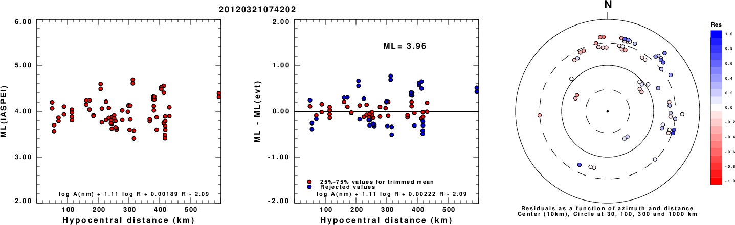
Left: ML computed using the IASPEI formula for Horizontal components. Center: ML residuals computed using a modified IASPEI formula that accounts for path specific attenuation; the values used for the trimmed mean are indicated. The ML relation used for each figure is given at the bottom of each plot.
Right: Residuals from new relation as a function of distance and azimuth.
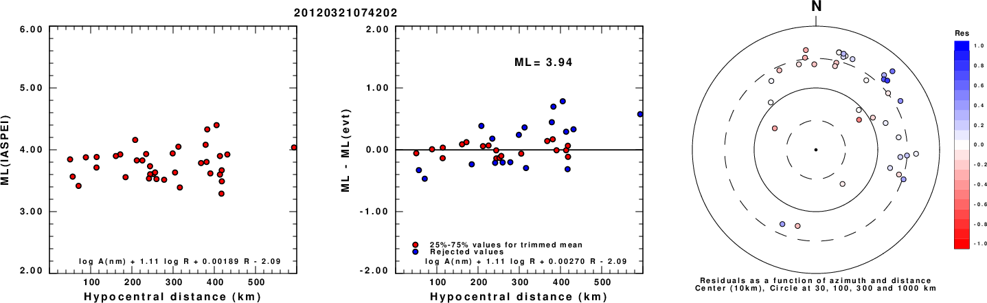
Left: ML computed using the IASPEI formula for Vertical components (research). Center: ML residuals computed using a modified IASPEI formula that accounts for path specific attenuation; the values used for the trimmed mean are indicated. The ML relation used for each figure is given at the bottom of each plot.
Right: Residuals from new relation as a function of distance and azimuth.
Context
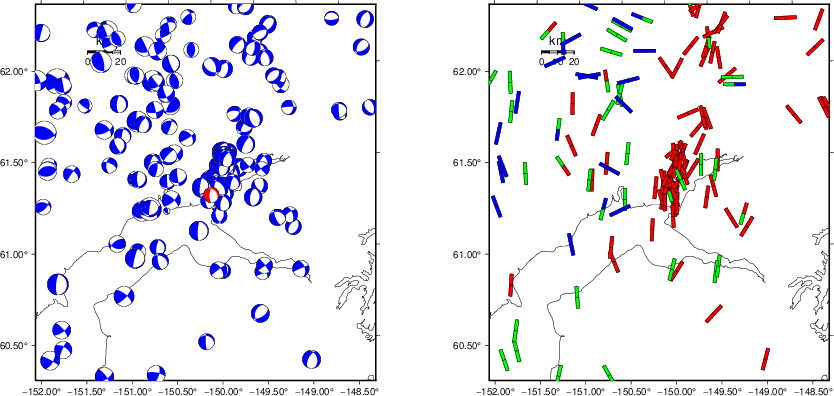
The left panel of the next figure presents the focal mechanism for this earthquake (red) in the context of other nearby events (blue) in the SLU Moment Tensor Catalog. The right panel shows the inferred direction of maximum compressive stress and the type of faulting (green is strike-slip, red is normal, blue is thrust; oblique is shown by a combination of colors). Thus context plot is useful for assessing the appropriateness of the moment tensor of this event.
Waveform Inversion using wvfgrd96
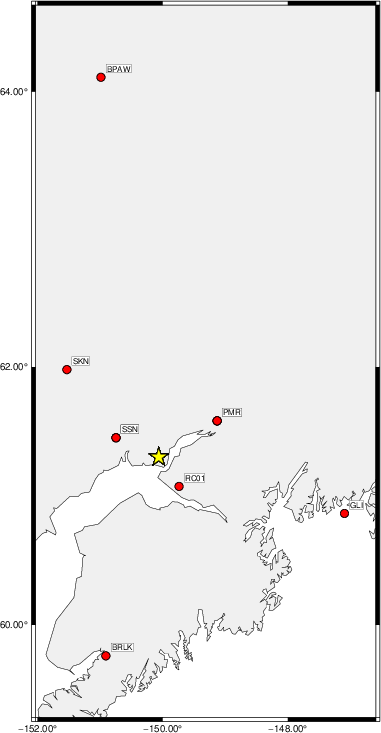
The focal mechanism was determined using broadband seismic waveforms. The location of the event (star) and the
stations used for (red) the waveform inversion are shown in the next figure.
|
|
Location of broadband stations used for waveform inversion
|
The program wvfgrd96 was used with good traces observed at short distance to determine the focal mechanism, depth and seismic moment. This technique requires a high quality signal and well determined velocity model for the Green's functions. To the extent that these are the quality data, this type of mechanism should be preferred over the radiation pattern technique which requires the separate step of defining the pressure and tension quadrants and the correct strike.
The observed and predicted traces are filtered using the following gsac commands:
hp c 0.02 n 3
lp c 0.10 n 3
br c 0.12 0.25 n 4 p 2
The results of this grid search are as follow:
           DEPTH  STK   DIP  RAKE   MW    FIT
WVFGRD96    0.5   215    45    85   3.00 0.1948
WVFGRD96    1.0   175    80    15   2.95 0.1447
WVFGRD96    2.0     5    40    90   3.17 0.2274
WVFGRD96    3.0   170    85   -25   3.20 0.2419
WVFGRD96    4.0   170    85   -30   3.26 0.2897
WVFGRD96    5.0   170    85   -35   3.30 0.3383
WVFGRD96    6.0   170    80   -35   3.33 0.3768
WVFGRD96    7.0   165    70   -40   3.35 0.4107
WVFGRD96    8.0   145    30    35   3.40 0.4308
WVFGRD96    9.0   145    30    35   3.40 0.4490
WVFGRD96   10.0   140    35    25   3.39 0.4604
WVFGRD96   11.0   140    35    25   3.39 0.4705
WVFGRD96   12.0   140    40    20   3.40 0.4793
WVFGRD96   13.0   140    40    20   3.41 0.4888
WVFGRD96   14.0   135    40    15   3.42 0.4969
WVFGRD96   15.0   135    40    15   3.43 0.5040
WVFGRD96   16.0   135    45    15   3.44 0.5100
WVFGRD96   17.0   135    45    10   3.45 0.5163
WVFGRD96   18.0   135    45    10   3.46 0.5209
WVFGRD96   19.0   135    45    10   3.47 0.5255
WVFGRD96   20.0   135    45    10   3.49 0.5289
WVFGRD96   21.0   135    45    10   3.50 0.5294
WVFGRD96   22.0   135    40    10   3.51 0.5308
WVFGRD96   23.0   160    40   -15   3.56 0.5370
WVFGRD96   24.0   160    40   -15   3.57 0.5420
WVFGRD96   25.0   160    40   -15   3.58 0.5461
WVFGRD96   26.0   160    40   -15   3.59 0.5494
WVFGRD96   27.0   165    45   -10   3.60 0.5514
WVFGRD96   28.0   160    40   -15   3.61 0.5545
WVFGRD96   29.0   160    45   -15   3.62 0.5592
WVFGRD96   30.0    30    85    70   3.58 0.5665
WVFGRD96   31.0    30    85    70   3.59 0.5714
WVFGRD96   32.0    30    85    70   3.59 0.5732
WVFGRD96   33.0   205    90   -65   3.60 0.5761
WVFGRD96   34.0    25    90    65   3.60 0.5783
WVFGRD96   35.0    25    90    65   3.61 0.5795
WVFGRD96   36.0    25    90    65   3.62 0.5802
WVFGRD96   37.0   200    85   -65   3.62 0.5834
WVFGRD96   38.0   195    80   -60   3.63 0.5824
WVFGRD96   39.0   195    80   -60   3.63 0.5820
WVFGRD96   40.0   195    80   -70   3.76 0.5716
WVFGRD96   41.0   195    80   -70   3.77 0.5765
WVFGRD96   42.0   195    80   -70   3.78 0.5816
WVFGRD96   43.0    55    15   -45   3.79 0.5858
WVFGRD96   44.0    65    20   -40   3.80 0.5899
WVFGRD96   45.0   185    70   -70   3.81 0.5975
WVFGRD96   46.0   180    65   -70   3.82 0.6014
WVFGRD96   47.0   185    70   -70   3.82 0.6058
WVFGRD96   48.0   180    65   -70   3.83 0.6080
WVFGRD96   49.0   185    70   -70   3.84 0.6108
WVFGRD96   50.0   185    70   -70   3.84 0.6108
WVFGRD96   51.0   185    70   -70   3.85 0.6111
WVFGRD96   52.0   185    70   -70   3.86 0.6099
WVFGRD96   53.0   185    70   -70   3.86 0.6074
WVFGRD96   54.0   180    70   -70   3.88 0.6048
WVFGRD96   55.0    20    15   -65   3.90 0.6029
WVFGRD96   56.0     0    15   -80   3.91 0.6046
WVFGRD96   57.0    -5    15   -85   3.92 0.6029
WVFGRD96   58.0     0    15   -80   3.92 0.6017
WVFGRD96   59.0    10    20   -70   3.92 0.6011
WVFGRD96   60.0    10    20   -70   3.93 0.5986
WVFGRD96   61.0    10    20   -70   3.93 0.5970
WVFGRD96   62.0    10    20   -70   3.94 0.5939
WVFGRD96   63.0    10    20   -70   3.94 0.5895
WVFGRD96   64.0    10    20   -70   3.94 0.5850
WVFGRD96   65.0    10    20   -70   3.95 0.5797
WVFGRD96   66.0    15    20   -65   3.95 0.5727
WVFGRD96   67.0    15    20   -65   3.95 0.5668
WVFGRD96   68.0    75    35   -60   3.93 0.5709
WVFGRD96   69.0    75    35   -60   3.93 0.5663
WVFGRD96   70.0    70    35   -60   3.93 0.5622
WVFGRD96   71.0    70    35   -60   3.93 0.5580
WVFGRD96   72.0    65    35   -65   3.92 0.5532
WVFGRD96   73.0    65    35   -65   3.92 0.5480
WVFGRD96   74.0    65    35   -65   3.93 0.5431
WVFGRD96   75.0   180    90   -70   4.01 0.5376
WVFGRD96   76.0   180    90   -70   4.01 0.5365
WVFGRD96   77.0     5    85    75   4.00 0.5390
WVFGRD96   78.0   180    90   -70   4.02 0.5330
WVFGRD96   79.0   180    90   -70   4.02 0.5308
WVFGRD96   80.0   180    90   -75   4.01 0.5291
WVFGRD96   81.0   180    90   -75   4.02 0.5266
WVFGRD96   82.0   180    90   -75   4.02 0.5243
WVFGRD96   83.0   180    90   -75   4.02 0.5219
WVFGRD96   84.0     0    85    75   4.01 0.5257
WVFGRD96   85.0   180    90   -75   4.02 0.5156
WVFGRD96   86.0   180    90   -75   4.02 0.5129
WVFGRD96   87.0     0    85    80   4.01 0.5182
WVFGRD96   88.0   145    40   -10   4.09 0.5190
WVFGRD96   89.0   145    40   -10   4.09 0.5167
WVFGRD96   90.0   145    45   -10   4.11 0.5145
WVFGRD96   91.0   145    45   -10   4.11 0.5139
WVFGRD96   92.0   145    45   -10   4.11 0.5124
WVFGRD96   93.0   145    45   -10   4.11 0.5106
WVFGRD96   94.0   145    45   -10   4.11 0.5081
WVFGRD96   95.0   145    45   -10   4.11 0.5054
WVFGRD96   96.0   145    45   -10   4.11 0.5037
WVFGRD96   97.0   145    45   -10   4.11 0.5016
WVFGRD96   98.0   145    45   -10   4.11 0.4989
WVFGRD96   99.0   145    45   -10   4.11 0.4958
The best solution is
WVFGRD96 51.0 185 70 -70 3.85 0.6111
The mechanism corresponding to the best fit is
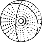
|
|
Figure 1. Waveform inversion focal mechanism
|
The best fit as a function of depth is given in the following figure:
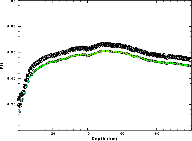
|
|
Figure 2. Depth sensitivity for waveform mechanism
|
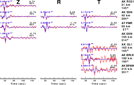
The comparison of the observed and predicted waveforms is given in the next figure. The red traces are the observed and the blue are the predicted.
Each observed-predicted component is plotted to the same scale and peak amplitudes are indicated by the numbers to the left of each trace. A pair of numbers is given in black at the right of each predicted traces. The upper number it the time shift required for maximum correlation between the observed and predicted traces. This time shift is required because the synthetics are not computed at exactly the same distance as the observed, the velocity model used in the predictions may not be perfect and the epicentral parameters may be be off.
A positive time shift indicates that the prediction is too fast and should be delayed to match the observed trace (shift to the right in this figure). A negative value indicates that the prediction is too slow. The lower number gives the percentage of variance reduction to characterize the individual goodness of fit (100% indicates a perfect fit).
The bandpass filter used in the processing and for the display was
hp c 0.02 n 3
lp c 0.10 n 3
br c 0.12 0.25 n 4 p 2
|
|
Figure 3. Waveform comparison for selected depth. Red: observed; Blue - predicted. The time shift with respect to the model prediction is indicated. The percent of fit is also indicated. The time scale is relative to the first trace sample.
|
|
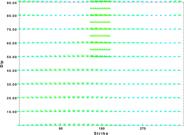
|
Focal mechanism sensitivity at the preferred depth. The red color indicates a very good fit to the waveforms.
Each solution is plotted as a vector at a given value of strike and dip with the angle of the vector representing the rake angle, measured, with respect to the upward vertical (N) in the figure.
|
A check on the assumed source location is possible by looking at the time shifts between the observed and predicted traces. The time shifts for waveform matching arise for several reasons:
- The origin time and epicentral distance are incorrect
- The velocity model used for the inversion is incorrect
- The velocity model used to define the P-arrival time is not the
same as the velocity model used for the waveform inversion
(assuming that the initial trace alignment is based on the
P arrival time)
Assuming only a mislocation, the time shifts are fit to a functional form:
Time_shift = A + B cos Azimuth + C Sin Azimuth
The time shifts for this inversion lead to the next figure:
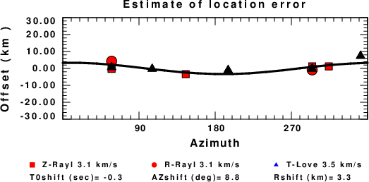
The derived shift in origin time and epicentral coordinates are given at the bottom of the figure.
Velocity Model
The WUS.model used for the waveform synthetic seismograms and for the surface wave eigenfunctions and dispersion is as follows
(The format is in the model96 format of Computer Programs in Seismology).
MODEL.01
Model after     8 iterations
ISOTROPIC
KGS
FLAT EARTH
1-D
CONSTANT VELOCITY
LINE08
LINE09
LINE10
LINE11
      H(KM)   VP(KM/S)   VS(KM/S) RHO(GM/CC)         QP         QS       ETAP       ETAS      FREFP      FREFS
     1.9000     3.4065     2.0089     2.2150  0.302E-02  0.679E-02   0.00       0.00       1.00       1.00
     6.1000     5.5445     3.2953     2.6089  0.349E-02  0.784E-02   0.00       0.00       1.00       1.00
    13.0000     6.2708     3.7396     2.7812  0.212E-02  0.476E-02   0.00       0.00       1.00       1.00
    19.0000     6.4075     3.7680     2.8223  0.111E-02  0.249E-02   0.00       0.00       1.00       1.00
     0.0000     7.9000     4.6200     3.2760  0.164E-10  0.370E-10   0.00       0.00       1.00       1.00
Last Changed Fri Apr 26 08:35:38 PM CDT 2024