Left: mLg computed using the IASPEI formula. Center: mLg residuals versus epicentral distance ; the values used for the trimmed mean magnitude estimate are indicated. Right: residuals as a function of distance and azimuth.
The ANSS event ID is nm609348 and the event page is at https://earthquake.usgs.gov/earthquakes/eventpage/nm609348/executive.
2012/02/21 09:58:43 36.873 -89.423 7.8 3.9 Missouri
 USGS/SLU Moment Tensor Solution
 ENS  2012/02/21 09:58:43:0  36.87  -89.42   7.8 3.9 Missouri

 Stations used:
   ET.FPAL IU.CCM IU.WCI IU.WVT NM.BLO NM.FVM NM.GLAT NM.GNAR
   NM.HALT NM.HBAR NM.LNXT NM.LPAR NM.MGMO NM.MPH NM.OLIL
   NM.PBMO NM.PEBM NM.PENM NM.PLAL NM.PVMO NM.SIUC NM.SLM
   NM.UALR NM.USIN NM.UTMT TA.147A TA.L40A TA.M42A TA.M44A
   TA.N38A TA.N39A TA.N40A TA.N41A TA.N42A TA.N46A TA.O37A
   TA.O38A TA.O39A TA.O40A TA.O41A TA.O42A TA.O43A TA.O44A
   TA.O45A TA.P38A TA.P39B TA.P40A TA.P41A TA.P42A TA.P43A
   TA.P44A TA.P46A TA.P47A TA.Q37A TA.Q38A TA.Q39A TA.Q40A
   TA.Q41A TA.Q42A TA.Q43A TA.Q44A TA.R36A TA.R37A TA.R38A
   TA.R39A TA.R40A TA.R41A TA.R42A TA.R43A TA.R44A TA.S37A
   TA.S38A TA.S39A TA.S40A TA.S41A TA.S42A TA.S43A TA.S44A
   TA.S45A TA.SFIN TA.T37A TA.T38A TA.T39A TA.T40A TA.T41A
   TA.T42A TA.T43A TA.TUL1 TA.U39A TA.U40A TA.U41A TA.U42A
   TA.U43A TA.U44A TA.U44B TA.U45A TA.V39A TA.V40A TA.V41A
   TA.V42A TA.V43A TA.V44A TA.V45A TA.W38A TA.W39A TA.W40A
   TA.W41B TA.W42A TA.W43A TA.W44A TA.W45A TA.X39A TA.X40A
   TA.X41A TA.X44A TA.X45A TA.Y40A TA.Y43A TA.Y44A TA.Y45A
   TA.Y46A TA.Y47A TA.Z44A TA.Z47A TA.Z48A US.HDIL US.LRAL
   US.OXF US.TZTN

 Filtering commands used:
   cut o DIST/3.3 -30 o DIST/3.3 +40
   rtr
   taper w 0.1
   hp c 0.03 n 3
   lp c 0.10 n 3

 Best Fitting Double Couple
  Mo = 9.55e+21 dyne-cm
  Mw = 3.92
  Z  = 10 km
  Plane   Strike  Dip  Rake
   NP1      250    73   -121
   NP2      135    35   -30
  Principal Axes:
   Axis    Value   Plunge  Azimuth
    T   9.55e+21     22       4
    N   0.00e+00     30     260
    P  -9.55e+21     51     124

 Moment Tensor: (dyne-cm)
    Component   Value
       Mxx     6.99e+21
       Mxy     2.24e+21
       Mxz     5.95e+21
       Myy    -2.50e+21
       Myz    -3.64e+21
       Mzz    -4.49e+21


                     ##############
                 ###########   ########
              ############## T ###########
             ###############   ############
           -#################################
          --##################################
         ---###################################
        ---########################-------------
        ----################--------------------
       -----###########--------------------------
       -----#######------------------------------
       ------###---------------------------------
       ------#---------------------   -----------
        ---####-------------------- P ----------
        -#######-------------------   ----------
         ########------------------------------
          #########---------------------------
           ##########------------------------
             ###########-------------------
              ###############-----------##
                 ######################
                     ##############


 Global CMT Convention Moment Tensor:
      R          T          P
 -4.49e+21   5.95e+21   3.64e+21
  5.95e+21   6.99e+21  -2.24e+21
  3.64e+21  -2.24e+21  -2.50e+21


Details of the solution is found at

http://www.eas.slu.edu/eqc/eqc_mt/MECH.NA/20120221095843/index.html
|
      STK = 135
      DIP = 35
     RAKE = -30
       MW = 3.92
       HS = 10.0
The NDK file is 20120221095843.ndk The waveform inversion is preferred.
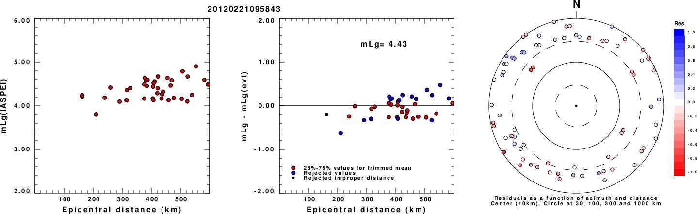
Given the availability of digital waveforms for determination of the moment tensor, this section documents the added processing leading to mLg, if appropriate to the region, and ML by application of the respective IASPEI formulae. As a research study, the linear distance term of the IASPEI formula for ML is adjusted to remove a linear distance trend in residuals to give a regionally defined ML. The defined ML uses horizontal component recordings, but the same procedure is applied to the vertical components since there may be some interest in vertical component ground motions. Residual plots versus distance may indicate interesting features of ground motion scaling in some distance ranges. A residual plot of the regionalized magnitude is given as a function of distance and azimuth, since data sets may transcend different wave propagation provinces.
Left: mLg computed using the IASPEI formula. Center: mLg residuals versus epicentral distance ; the values used for the trimmed mean magnitude estimate are indicated.
Right: residuals as a function of distance and azimuth.
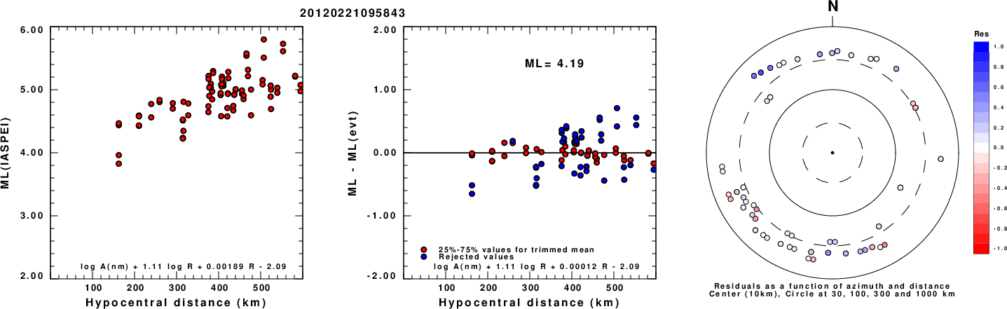
Left: ML computed using the IASPEI formula for Horizontal components. Center: ML residuals computed using a modified IASPEI formula that accounts for path specific attenuation; the values used for the trimmed mean are indicated. The ML relation used for each figure is given at the bottom of each plot.
Right: Residuals from new relation as a function of distance and azimuth.
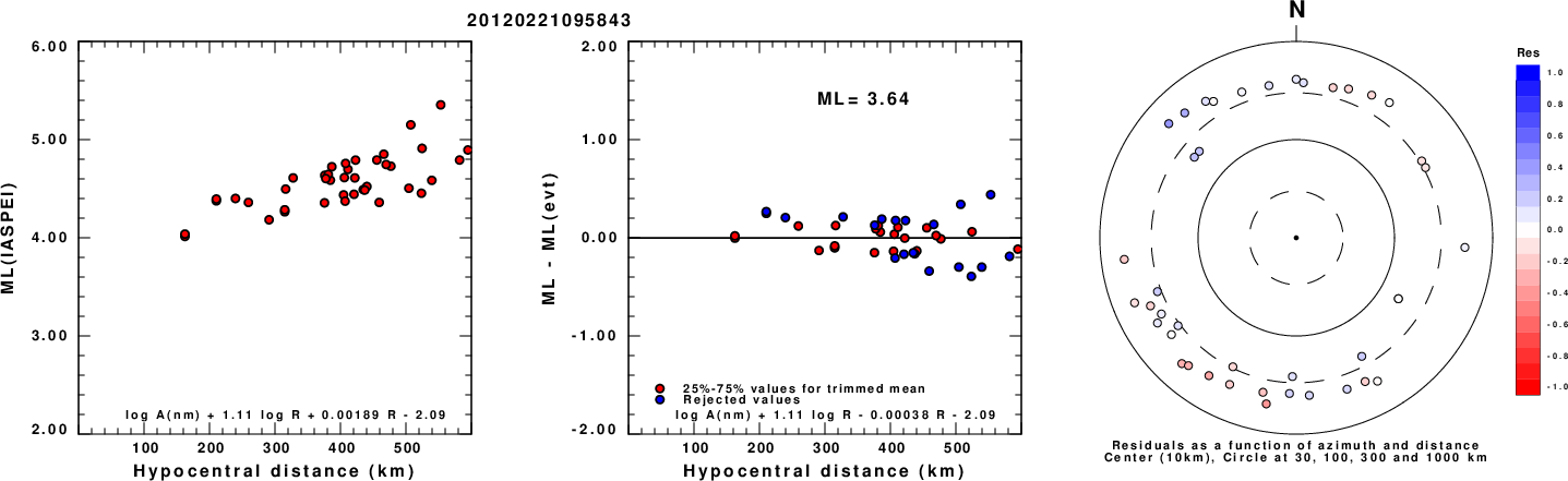
Left: ML computed using the IASPEI formula for Vertical components (research). Center: ML residuals computed using a modified IASPEI formula that accounts for path specific attenuation; the values used for the trimmed mean are indicated. The ML relation used for each figure is given at the bottom of each plot.
Right: Residuals from new relation as a function of distance and azimuth.
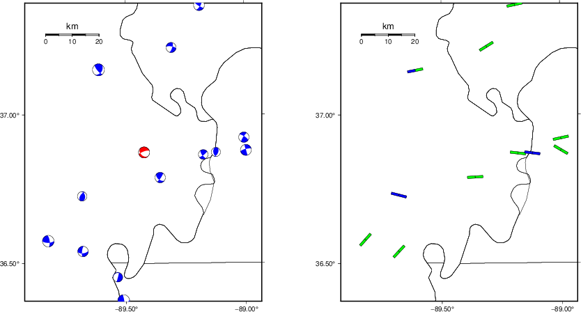 |
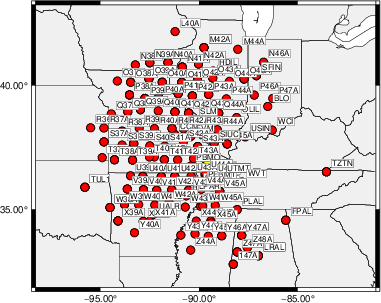
The focal mechanism was determined using broadband seismic waveforms. The location of the event (star) and the stations used for (red) the waveform inversion are shown in the next figure.
|
|
|
The program wvfgrd96 was used with good traces observed at short distance to determine the focal mechanism, depth and seismic moment. This technique requires a high quality signal and well determined velocity model for the Green's functions. To the extent that these are the quality data, this type of mechanism should be preferred over the radiation pattern technique which requires the separate step of defining the pressure and tension quadrants and the correct strike.
The observed and predicted traces are filtered using the following gsac commands:
cut o DIST/3.3 -30 o DIST/3.3 +40
rtr
taper w 0.1
hp c 0.03 n 3
lp c 0.10 n 3
The results of this grid search are as follow:
           DEPTH  STK   DIP  RAKE   MW    FIT
WVFGRD96    0.5   305    40   -20   3.83 0.4650
WVFGRD96    1.0   305    40   -25   3.85 0.4679
WVFGRD96    2.0   150    25     0   3.92 0.4721
WVFGRD96    3.0   155    30     5   3.89 0.5199
WVFGRD96    4.0   155    30     5   3.87 0.5596
WVFGRD96    5.0   160    35    15   3.88 0.5906
WVFGRD96    6.0   160    40    20   3.89 0.6120
WVFGRD96    7.0   160    40    20   3.89 0.6256
WVFGRD96    8.0   135    35   -35   3.89 0.6344
WVFGRD96    9.0   135    35   -35   3.89 0.6399
WVFGRD96   10.0   135    35   -30   3.92 0.6408
WVFGRD96   11.0   130    35   -40   3.93 0.6376
WVFGRD96   12.0   130    35   -40   3.93 0.6303
WVFGRD96   13.0   130    35   -35   3.94 0.6202
WVFGRD96   14.0   130    35   -35   3.94 0.6075
WVFGRD96   15.0   130    35   -35   3.95 0.5929
WVFGRD96   16.0   130    35   -35   3.96 0.5770
WVFGRD96   17.0   130    35   -35   3.96 0.5598
WVFGRD96   18.0   125    30   -45   3.96 0.5422
WVFGRD96   19.0   125    30   -45   3.97 0.5246
WVFGRD96   20.0   125    30   -45   4.00 0.5088
WVFGRD96   21.0   130    30   -40   4.01 0.4895
WVFGRD96   22.0   130    30   -40   4.01 0.4705
WVFGRD96   23.0   120    30   -50   4.02 0.4527
WVFGRD96   24.0   120    30   -50   4.03 0.4351
WVFGRD96   25.0   120    30   -50   4.03 0.4180
WVFGRD96   26.0   125    30   -45   4.04 0.4011
WVFGRD96   27.0   125    30   -45   4.04 0.3842
WVFGRD96   28.0   125    30   -45   4.05 0.3673
WVFGRD96   29.0   130    30   -35   4.05 0.3510
The best solution is
WVFGRD96 10.0 135 35 -30 3.92 0.6408
The mechanism corresponding to the best fit is
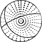
|
|
|
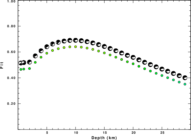
The best fit as a function of depth is given in the following figure:
|
|
|
The comparison of the observed and predicted waveforms is given in the next figure. The red traces are the observed and the blue are the predicted. Each observed-predicted component is plotted to the same scale and peak amplitudes are indicated by the numbers to the left of each trace. A pair of numbers is given in black at the right of each predicted traces. The upper number it the time shift required for maximum correlation between the observed and predicted traces. This time shift is required because the synthetics are not computed at exactly the same distance as the observed, the velocity model used in the predictions may not be perfect and the epicentral parameters may be be off. A positive time shift indicates that the prediction is too fast and should be delayed to match the observed trace (shift to the right in this figure). A negative value indicates that the prediction is too slow. The lower number gives the percentage of variance reduction to characterize the individual goodness of fit (100% indicates a perfect fit).
The bandpass filter used in the processing and for the display was
cut o DIST/3.3 -30 o DIST/3.3 +40
rtr
taper w 0.1
hp c 0.03 n 3
lp c 0.10 n 3

|
| Figure 3. Waveform comparison for selected depth. Red: observed; Blue - predicted. The time shift with respect to the model prediction is indicated. The percent of fit is also indicated. The time scale is relative to the first trace sample. |
|
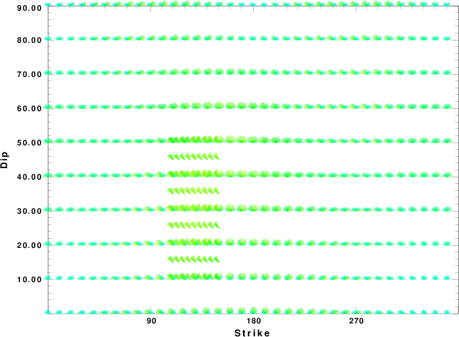
| Focal mechanism sensitivity at the preferred depth. The red color indicates a very good fit to the waveforms. Each solution is plotted as a vector at a given value of strike and dip with the angle of the vector representing the rake angle, measured, with respect to the upward vertical (N) in the figure. |
A check on the assumed source location is possible by looking at the time shifts between the observed and predicted traces. The time shifts for waveform matching arise for several reasons:
Time_shift = A + B cos Azimuth + C Sin Azimuth
The time shifts for this inversion lead to the next figure:
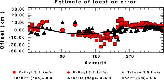
The derived shift in origin time and epicentral coordinates are given at the bottom of the figure.
The CUS.model used for the waveform synthetic seismograms and for the surface wave eigenfunctions and dispersion is as follows (The format is in the model96 format of Computer Programs in Seismology).
MODEL.01
CUS Model with Q from simple gamma values
ISOTROPIC
KGS
FLAT EARTH
1-D
CONSTANT VELOCITY
LINE08
LINE09
LINE10
LINE11
  H(KM) VP(KM/S) VS(KM/S) RHO(GM/CC)   QP   QS  ETAP  ETAS  FREFP  FREFS
  1.0000  5.0000  2.8900  2.5000 0.172E-02 0.387E-02 0.00  0.00  1.00  1.00
  9.0000  6.1000  3.5200  2.7300 0.160E-02 0.363E-02 0.00  0.00  1.00  1.00
 10.0000  6.4000  3.7000  2.8200 0.149E-02 0.336E-02 0.00  0.00  1.00  1.00
 20.0000  6.7000  3.8700  2.9020 0.000E-04 0.000E-04 0.00  0.00  1.00  1.00
  0.0000  8.1500  4.7000  3.3640 0.194E-02 0.431E-02 0.00  0.00  1.00  1.00