Location
Location ANSS
The ANSS event ID is usp000jajb and the event page is at
https://earthquake.usgs.gov/earthquakes/eventpage/usp000jajb/executive.
2011/11/08 02:46:57 35.531 -96.788 5.0 4.8 Oklahoma
Focal Mechanism
 USGS/SLU Moment Tensor Solution
 ENS  2011/11/08 02:46:57:0  35.53  -96.79   5.0 4.8 Oklahoma

 Stations used:
   AG.FCAR AG.HHAR AG.LCAR AG.WLAR IU.CCM NM.MGMO NM.PBMO
   NM.UALR NM.X301 TA.136A TA.137A TA.138A TA.139A TA.141A
   TA.236A TA.237A TA.238A TA.338A TA.436A TA.ABTX TA.MSTX
   TA.N33A TA.O33A TA.O34A TA.O36A TA.O37A TA.O38A TA.P34A
   TA.P36A TA.P37A TA.P38A TA.P39B TA.Q34A TA.Q35A TA.Q36A
   TA.Q37A TA.Q38A TA.Q39A TA.Q40A TA.R34A TA.R35A TA.R36A
   TA.R37A TA.R38A TA.R39A TA.R40A TA.R41A TA.S34A TA.S35A
   TA.S36A TA.S37A TA.S38A TA.S39A TA.S40A TA.S41A TA.S42A
   TA.T34A TA.T35A TA.T36A TA.T37A TA.T38A TA.T39A TA.T40A
   TA.T41A TA.TUL1 TA.U32A TA.U35A TA.U36A TA.U37A TA.U38A
   TA.U39A TA.U40A TA.U41A TA.V36A TA.V37A TA.V38A TA.V39A
   TA.V40A TA.V41A TA.V42A TA.W35A TA.W36A TA.W37B TA.W38A
   TA.W39A TA.W40A TA.W42A TA.WHTX TA.X35A TA.X36A TA.X37A
   TA.X38A TA.X39A TA.X40A TA.X41A TA.Y35A TA.Y36A TA.Y37A
   TA.Y38A TA.Y39A TA.Y40A TA.Y41A TA.Y43A TA.Z36A TA.Z37A
   TA.Z38A TA.Z39A TA.Z40A TA.Z41A US.CBKS US.KSU1 US.MIAR
   US.WMOK

 Filtering commands used:
   hp c 0.02 n 3
   lp c 0.06 n 3

 Best Fitting Double Couple
  Mo = 2.21e+23 dyne-cm
  Mw = 4.83
  Z  = 8 km
  Plane   Strike  Dip  Rake
   NP1       95    90   -15
   NP2      185    75   -180
  Principal Axes:
   Axis    Value   Plunge  Azimuth
    T   2.21e+23     11     141
    N   0.00e+00     75     275
    P  -2.21e+23     11      49

 Moment Tensor: (dyne-cm)
    Component   Value
       Mxx     3.71e+22
       Mxy    -2.11e+23
       Mxz    -5.71e+22
       Myy    -3.71e+22
       Myz    -4.99e+21
       Mzz     5.01e+15


                     ########------
                 ###########-----------
              #############---------------
             ##############--------------
           ###############--------------- P -
          ################---------------   --
         ################----------------------
        #################-----------------------
        #################-----------------------
       #################-------------------------
       ----------#######-------------------------
       -----------------###############----------
       -----------------#########################
        ----------------########################
        ----------------########################
         ---------------#######################
          --------------######################
           -------------###############   ###
             -----------############### T #
              -----------##############
                 --------##############
                     -----#########


 Global CMT Convention Moment Tensor:
      R          T          P
  5.01e+15  -5.71e+22   4.99e+21
 -5.71e+22   3.71e+22   2.11e+23
  4.99e+21   2.11e+23  -3.71e+22


Details of the solution is found at

http://www.eas.slu.edu/eqc/eqc_mt/MECH.NA/20111108024657/index.html
|
Preferred Solution
The preferred solution from an analysis of the surface-wave spectral amplitude radiation pattern, waveform inversion or first motion observations is
      STK = 95
      DIP = 90
     RAKE = -15
       MW = 4.83
       HS = 8.0
The NDK file is 20111108024657.ndk
The waveform inversion is preferred.
Moment Tensor Comparison
The following compares this source inversion to those provided by others. The purpose is to look for major differences and also to note slight differences that might be inherent to the processing procedure. For completeness the USGS/SLU solution is repeated from above.
| SLU |
USGSMT |
GCMT |
 USGS/SLU Moment Tensor Solution
 ENS  2011/11/08 02:46:57:0  35.53  -96.79   5.0 4.8 Oklahoma

 Stations used:
   AG.FCAR AG.HHAR AG.LCAR AG.WLAR IU.CCM NM.MGMO NM.PBMO
   NM.UALR NM.X301 TA.136A TA.137A TA.138A TA.139A TA.141A
   TA.236A TA.237A TA.238A TA.338A TA.436A TA.ABTX TA.MSTX
   TA.N33A TA.O33A TA.O34A TA.O36A TA.O37A TA.O38A TA.P34A
   TA.P36A TA.P37A TA.P38A TA.P39B TA.Q34A TA.Q35A TA.Q36A
   TA.Q37A TA.Q38A TA.Q39A TA.Q40A TA.R34A TA.R35A TA.R36A
   TA.R37A TA.R38A TA.R39A TA.R40A TA.R41A TA.S34A TA.S35A
   TA.S36A TA.S37A TA.S38A TA.S39A TA.S40A TA.S41A TA.S42A
   TA.T34A TA.T35A TA.T36A TA.T37A TA.T38A TA.T39A TA.T40A
   TA.T41A TA.TUL1 TA.U32A TA.U35A TA.U36A TA.U37A TA.U38A
   TA.U39A TA.U40A TA.U41A TA.V36A TA.V37A TA.V38A TA.V39A
   TA.V40A TA.V41A TA.V42A TA.W35A TA.W36A TA.W37B TA.W38A
   TA.W39A TA.W40A TA.W42A TA.WHTX TA.X35A TA.X36A TA.X37A
   TA.X38A TA.X39A TA.X40A TA.X41A TA.Y35A TA.Y36A TA.Y37A
   TA.Y38A TA.Y39A TA.Y40A TA.Y41A TA.Y43A TA.Z36A TA.Z37A
   TA.Z38A TA.Z39A TA.Z40A TA.Z41A US.CBKS US.KSU1 US.MIAR
   US.WMOK

 Filtering commands used:
   hp c 0.02 n 3
   lp c 0.06 n 3

 Best Fitting Double Couple
  Mo = 2.21e+23 dyne-cm
  Mw = 4.83
  Z  = 8 km
  Plane   Strike  Dip  Rake
   NP1       95    90   -15
   NP2      185    75   -180
  Principal Axes:
   Axis    Value   Plunge  Azimuth
    T   2.21e+23     11     141
    N   0.00e+00     75     275
    P  -2.21e+23     11      49

 Moment Tensor: (dyne-cm)
    Component   Value
       Mxx     3.71e+22
       Mxy    -2.11e+23
       Mxz    -5.71e+22
       Myy    -3.71e+22
       Myz    -4.99e+21
       Mzz     5.01e+15


                     ########------
                 ###########-----------
              #############---------------
             ##############--------------
           ###############--------------- P -
          ################---------------   --
         ################----------------------
        #################-----------------------
        #################-----------------------
       #################-------------------------
       ----------#######-------------------------
       -----------------###############----------
       -----------------#########################
        ----------------########################
        ----------------########################
         ---------------#######################
          --------------######################
           -------------###############   ###
             -----------############### T #
              -----------##############
                 --------##############
                     -----#########


 Global CMT Convention Moment Tensor:
      R          T          P
  5.01e+15  -5.71e+22   4.99e+21
 -5.71e+22   3.71e+22   2.11e+23
  4.99e+21   2.11e+23  -3.71e+22


Details of the solution is found at

http://www.eas.slu.edu/eqc/eqc_mt/MECH.NA/20111108024657/index.html
|
USGS/SLU Regional Moment Solution
OKLAHOMA

11/11/08 02:46:57.04

Epicenter:  35.535  -96.779
MW 4.8

USGS/SLU REGIONAL MOMENT TENSOR
Depth   6         No. of sta: 57
Moment Tensor;   Scale 10**16 Nm
  Mrr=-0.25       Mtt= 0.39
  Mpp=-0.13       Mrt= 0.15
  Mrp= 0.50       Mtp= 2.01
 Principal axes:
  T  Val=  2.23  Plg=10  Azm=318
  N       -0.29      76      181
  P       -1.95       9       50

Best Double Couple:Mo=2.1*10**16
 NP1:Strike= 94 Dip=76 Slip=   1
 NP2:         4     89       166

|
ovember 8, 2011, OKLAHOMA, MW=5.0

Meredith Nettles
Goran Ekstrom

CENTROID-MOMENT-TENSOR  SOLUTION
GCMT EVENT:     C201111080246A
DATA: DK CU IU G  II LD GE
L.P.BODY WAVES: 18S,  19C, T= 40
SURFACE WAVES:  38S,  76C, T= 50
TIMESTAMP:      Q-20111108172407
CENTROID LOCATION:
ORIGIN TIME:      02:46:59.0 0.3
LAT:35.56N 0.02;LON: 96.75W 0.02
DEP: 12.0  FIX;TRIANG HDUR:  0.8
MOMENT TENSOR: SCALE 10**23 D-CM
RR= 0.119 0.131; TT= 0.061 0.139
PP=-0.179 0.106; RT= 0.548 0.364
RP=-0.424 0.329; TP= 3.320 0.093
PRINCIPAL AXES:
1.(T) VAL=  3.266;PLG= 2;AZM=316
2.(N)       0.245;    79;     56
3.(P)      -3.511;    11;    226
BEST DBLE.COUPLE:M0= 3.39*10**23
NP1: STRIKE=  2;DIP=81;SLIP=-174
NP2: STRIKE=271;DIP=84;SLIP=  -9

            ######-----
        ###########--------
      T ###########----------
    #   ###########------------
   ################-------------
  #################--------------
  #################--------------
 ##################---------------
 ######------------#######--------
 ------------------###############
 ------------------###############
  -----------------##############
  -----------------##############
   --   -----------#############
    - P ----------#############
        ----------###########
        ----------#########
            -----######
|
Magnitudes
Given the availability of digital waveforms for determination of the moment tensor, this section documents the added processing leading to mLg, if appropriate to the region, and ML by application of the respective IASPEI formulae. As a research study, the linear distance term of the IASPEI formula
for ML is adjusted to remove a linear distance trend in residuals to give a regionally defined ML. The defined ML uses horizontal component recordings, but the same procedure is applied to the vertical components since there may be some interest in vertical component ground motions. Residual plots versus distance may indicate interesting features of ground motion scaling in some distance ranges. A residual plot of the regionalized magnitude is given as a function of distance and azimuth, since data sets may transcend different wave propagation provinces.
mLg Magnitude
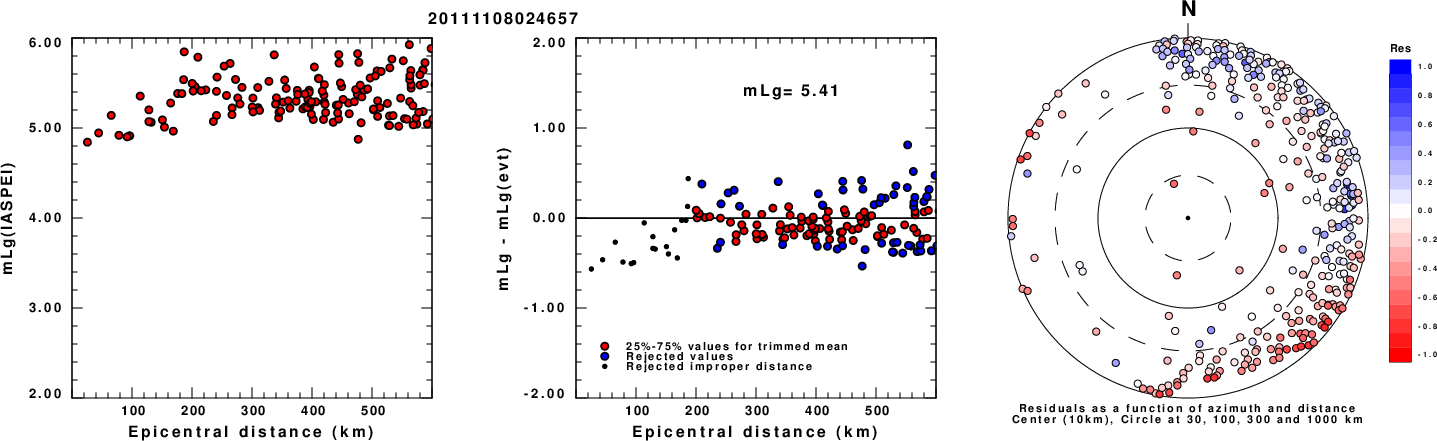
Left: mLg computed using the IASPEI formula. Center: mLg residuals versus epicentral distance ; the values used for the trimmed mean magnitude estimate are indicated.
Right: residuals as a function of distance and azimuth.
ML Magnitude
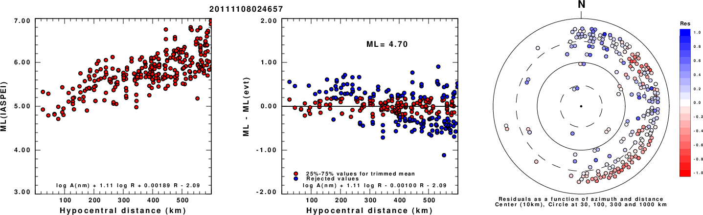
Left: ML computed using the IASPEI formula for Horizontal components. Center: ML residuals computed using a modified IASPEI formula that accounts for path specific attenuation; the values used for the trimmed mean are indicated. The ML relation used for each figure is given at the bottom of each plot.
Right: Residuals from new relation as a function of distance and azimuth.
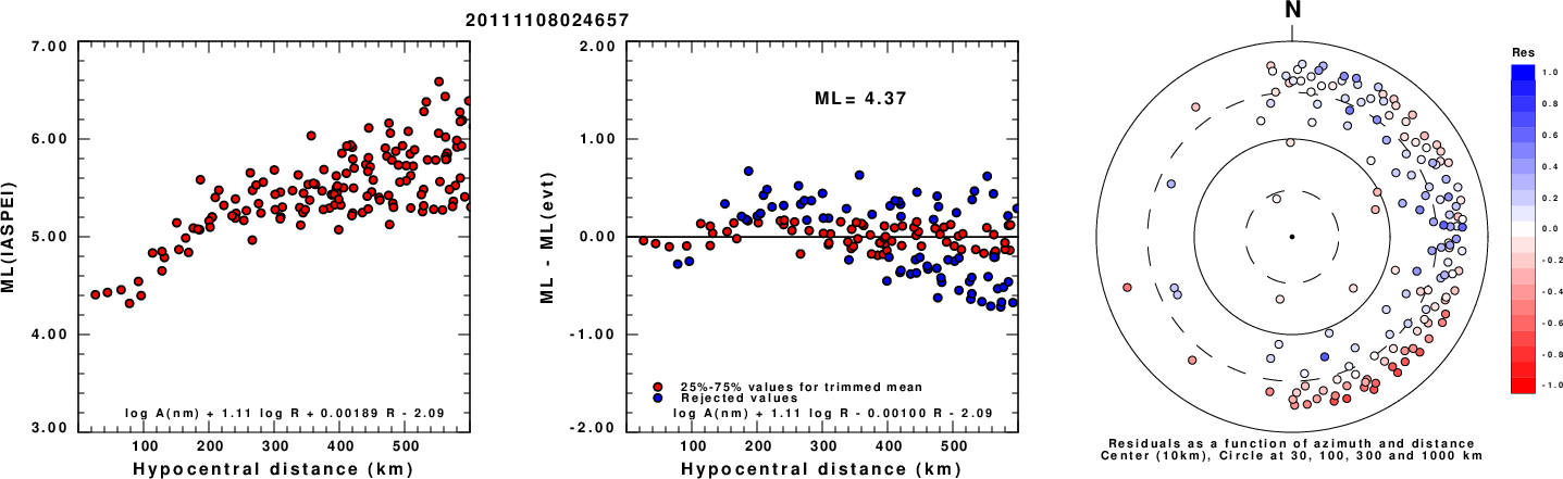
Left: ML computed using the IASPEI formula for Vertical components (research). Center: ML residuals computed using a modified IASPEI formula that accounts for path specific attenuation; the values used for the trimmed mean are indicated. The ML relation used for each figure is given at the bottom of each plot.
Right: Residuals from new relation as a function of distance and azimuth.
Context
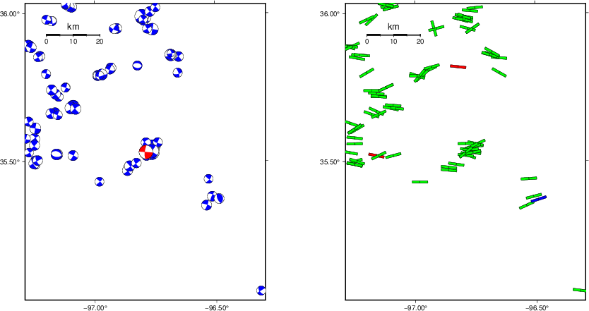
The left panel of the next figure presents the focal mechanism for this earthquake (red) in the context of other nearby events (blue) in the SLU Moment Tensor Catalog. The right panel shows the inferred direction of maximum compressive stress and the type of faulting (green is strike-slip, red is normal, blue is thrust; oblique is shown by a combination of colors). Thus context plot is useful for assessing the appropriateness of the moment tensor of this event.
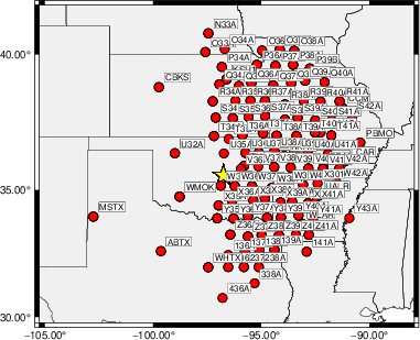
Waveform Inversion using wvfgrd96
The focal mechanism was determined using broadband seismic waveforms. The location of the event (star) and the
stations used for (red) the waveform inversion are shown in the next figure.
|
|
Location of broadband stations used for waveform inversion
|
The program wvfgrd96 was used with good traces observed at short distance to determine the focal mechanism, depth and seismic moment. This technique requires a high quality signal and well determined velocity model for the Green's functions. To the extent that these are the quality data, this type of mechanism should be preferred over the radiation pattern technique which requires the separate step of defining the pressure and tension quadrants and the correct strike.
The observed and predicted traces are filtered using the following gsac commands:
hp c 0.02 n 3
lp c 0.06 n 3
The results of this grid search are as follow:
           DEPTH  STK   DIP  RAKE   MW    FIT
WVFGRD96    0.5   270    75   -20   4.54 0.4186
WVFGRD96    1.0   275    85    -5   4.55 0.4517
WVFGRD96    2.0   270    75   -20   4.67 0.5566
WVFGRD96    3.0   275    90     0   4.69 0.6021
WVFGRD96    4.0   275    90     0   4.73 0.6243
WVFGRD96    5.0   275    85     5   4.75 0.6333
WVFGRD96    6.0    95    90    -5   4.78 0.6360
WVFGRD96    7.0    95    90   -10   4.80 0.6365
WVFGRD96    8.0    95    90   -15   4.83 0.6378
WVFGRD96    9.0    95    90   -15   4.84 0.6259
WVFGRD96   10.0   275    70     5   4.85 0.6166
WVFGRD96   11.0   275    70     5   4.86 0.6082
WVFGRD96   12.0    95    70     5   4.87 0.6046
WVFGRD96   13.0    95    70     5   4.88 0.5991
WVFGRD96   14.0    95    70     5   4.89 0.5928
WVFGRD96   15.0    95    70     5   4.90 0.5856
WVFGRD96   16.0    95    70     5   4.90 0.5776
WVFGRD96   17.0    95    70     5   4.91 0.5691
WVFGRD96   18.0    95    70     5   4.91 0.5605
WVFGRD96   19.0    95    70     5   4.92 0.5517
WVFGRD96   20.0    95    75    -5   4.93 0.5429
WVFGRD96   21.0    95    75    -5   4.94 0.5353
WVFGRD96   22.0    95    75    -5   4.94 0.5274
WVFGRD96   23.0    95    75    -5   4.95 0.5194
WVFGRD96   24.0    95    75    -5   4.95 0.5112
WVFGRD96   25.0    95    75    -5   4.96 0.5034
WVFGRD96   26.0    95    75    -5   4.96 0.4956
WVFGRD96   27.0    95    75    -5   4.97 0.4877
WVFGRD96   28.0    95    75    -5   4.98 0.4803
WVFGRD96   29.0    95    75    -5   4.98 0.4728
The best solution is
WVFGRD96 8.0 95 90 -15 4.83 0.6378
The mechanism corresponding to the best fit is
|
|
Figure 1. Waveform inversion focal mechanism
|
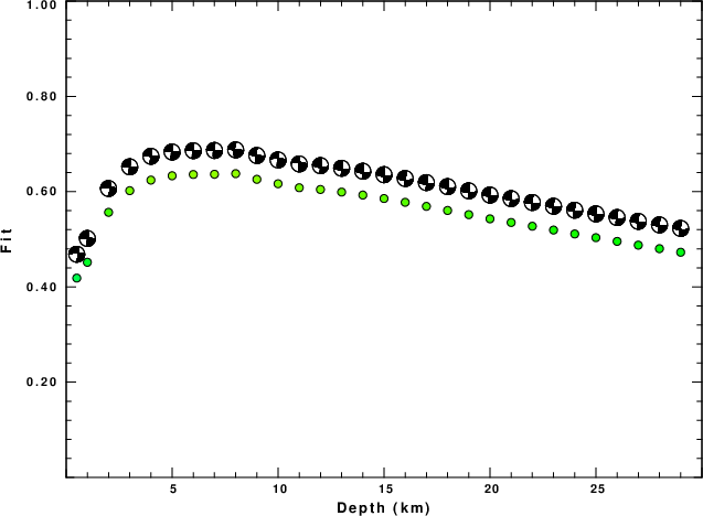
The best fit as a function of depth is given in the following figure:
|
|
Figure 2. Depth sensitivity for waveform mechanism
|
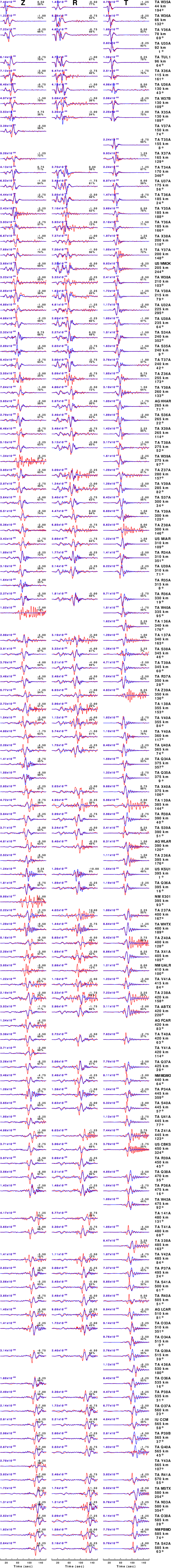
The comparison of the observed and predicted waveforms is given in the next figure. The red traces are the observed and the blue are the predicted.
Each observed-predicted component is plotted to the same scale and peak amplitudes are indicated by the numbers to the left of each trace. A pair of numbers is given in black at the right of each predicted traces. The upper number it the time shift required for maximum correlation between the observed and predicted traces. This time shift is required because the synthetics are not computed at exactly the same distance as the observed, the velocity model used in the predictions may not be perfect and the epicentral parameters may be be off.
A positive time shift indicates that the prediction is too fast and should be delayed to match the observed trace (shift to the right in this figure). A negative value indicates that the prediction is too slow. The lower number gives the percentage of variance reduction to characterize the individual goodness of fit (100% indicates a perfect fit).
The bandpass filter used in the processing and for the display was
hp c 0.02 n 3
lp c 0.06 n 3
|
|
Figure 3. Waveform comparison for selected depth. Red: observed; Blue - predicted. The time shift with respect to the model prediction is indicated. The percent of fit is also indicated. The time scale is relative to the first trace sample.
|
|
|
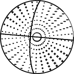
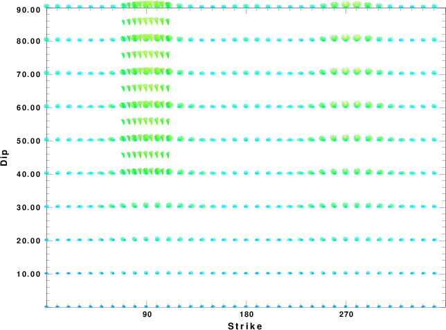
Focal mechanism sensitivity at the preferred depth. The red color indicates a very good fit to the waveforms.
Each solution is plotted as a vector at a given value of strike and dip with the angle of the vector representing the rake angle, measured, with respect to the upward vertical (N) in the figure.
|
A check on the assumed source location is possible by looking at the time shifts between the observed and predicted traces. The time shifts for waveform matching arise for several reasons:
- The origin time and epicentral distance are incorrect
- The velocity model used for the inversion is incorrect
- The velocity model used to define the P-arrival time is not the
same as the velocity model used for the waveform inversion
(assuming that the initial trace alignment is based on the
P arrival time)
Assuming only a mislocation, the time shifts are fit to a functional form:
Time_shift = A + B cos Azimuth + C Sin Azimuth
The time shifts for this inversion lead to the next figure:
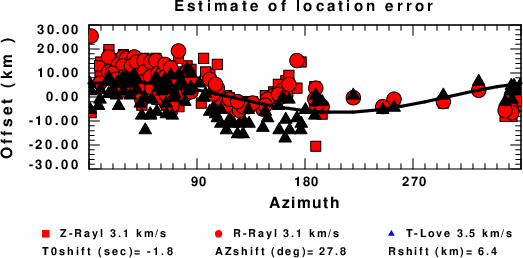
The derived shift in origin time and epicentral coordinates are given at the bottom of the figure.
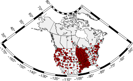
Surface-Wave Focal Mechanism
The following figure shows the stations used in the grid search for the best focal mechanism to fit the surface-wave spectral amplitudes of the Love and Rayleigh waves.
|
|
Location of broadband stations used to obtain focal mechanism from surface-wave spectral amplitudes
|
The surface-wave determined focal mechanism is shown here.
  NODAL PLANES


  STK=       5.00
  DIP=      90.00
 RAKE=    -160.00

             OR

  STK=     275.00
  DIP=      70.00
 RAKE=      -0.01


DEPTH = 5.0 km

Mw = 4.92
Best Fit 0.8634 - P-T axis plot gives solutions with FIT greater than FIT90
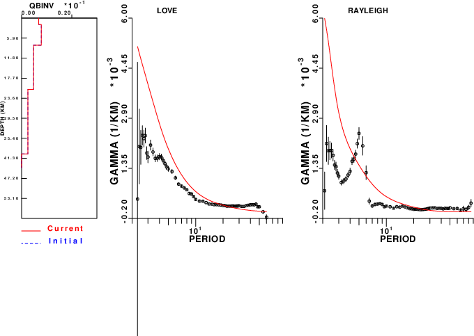
Surface-wave analysis
Surface wave analysis was performed using codes from
Computer Programs in Seismology, specifically the
multiple filter analysis program do_mft and the surface-wave
radiation pattern search program srfgrd96.
Data preparation
Digital data were collected, instrument response removed and traces converted
to Z, R an T components. Multiple filter analysis was applied to the Z and T traces to obtain the Rayleigh- and Love-wave spectral amplitudes, respectively.
These were input to the search program which examined all depths between 1 and 25 km
and all possible mechanisms.
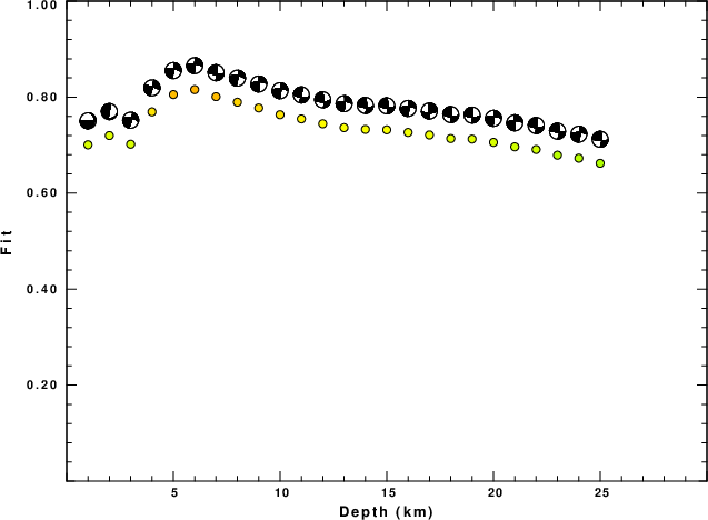
|
|
Best mechanism fit as a function of depth. The preferred depth is given above. Lower hemisphere projection
|
|
|
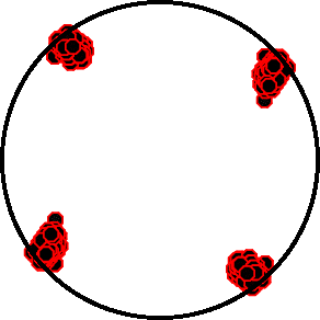
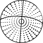
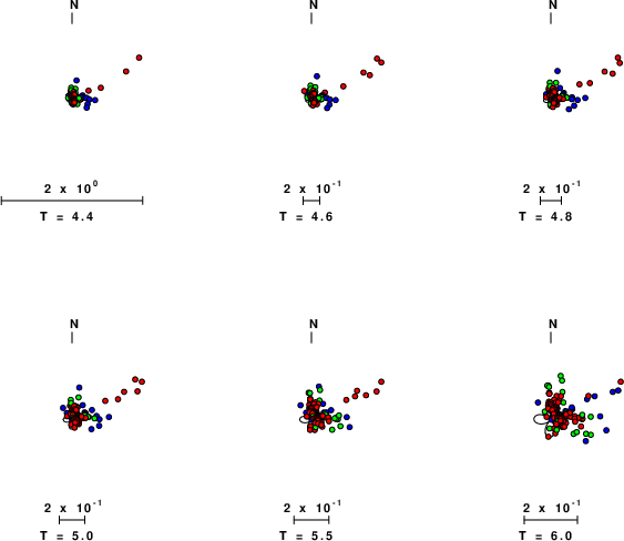
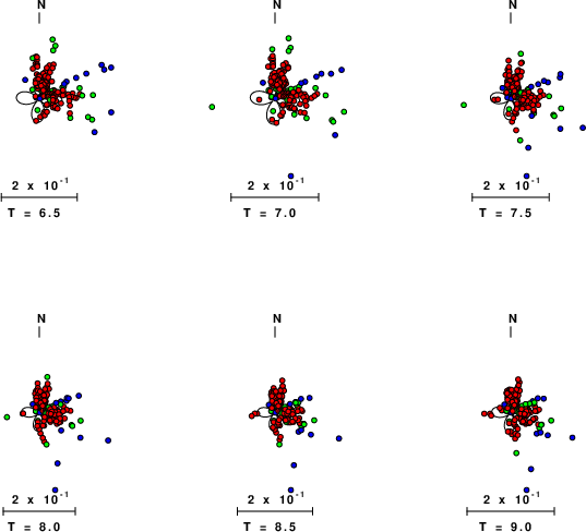
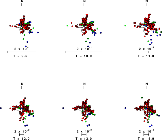
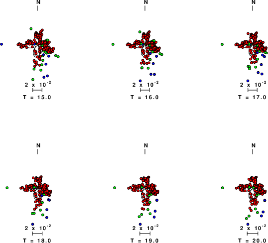
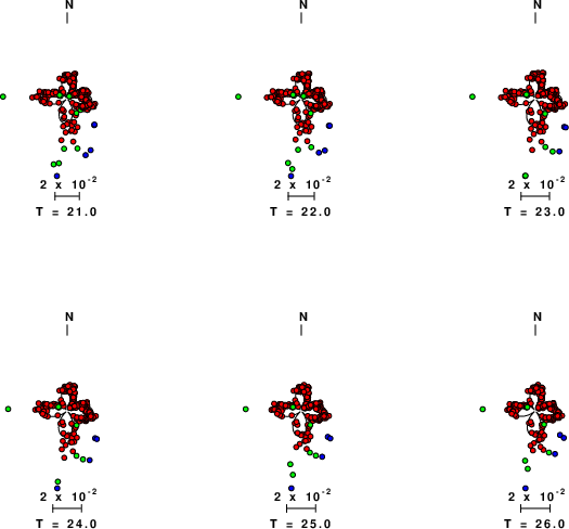
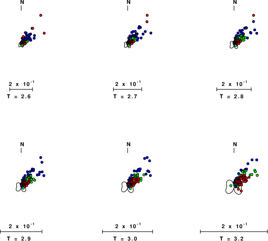
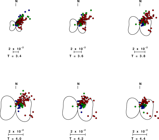
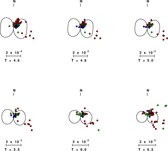
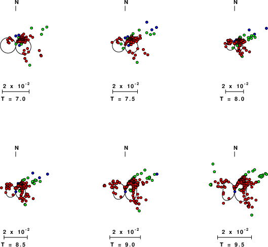
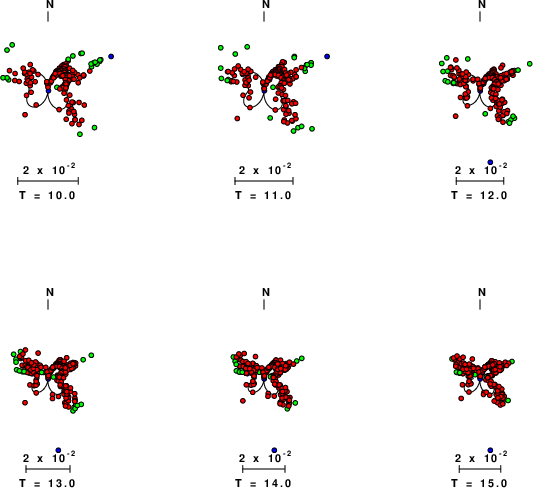
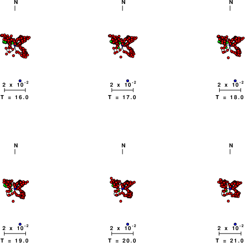
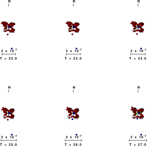
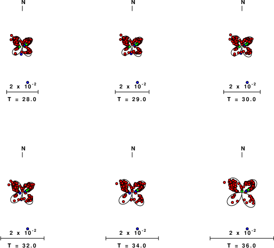
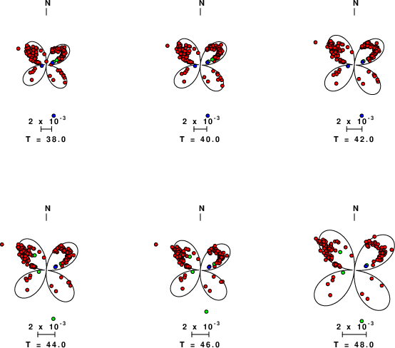
Pressure-tension axis trends. Since the surface-wave spectra search does not distinguish between P and T axes and since there is a 180 ambiguity in strike, all possible P and T axes are plotted. First motion data and waveforms will be used to select the preferred mechanism. The purpose of this plot is to provide an idea of the
possible range of solutions. The P and T-axes for all mechanisms with goodness of fit greater than 0.9 FITMAX (above) are plotted here.
|
|
|
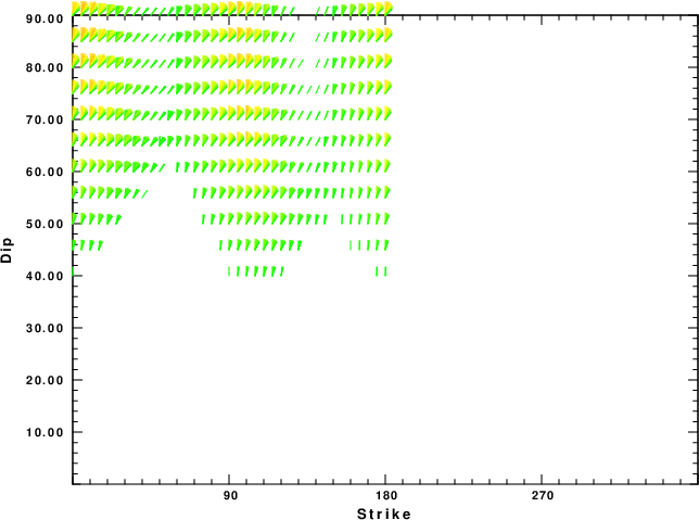
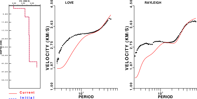
Focal mechanism sensitivity at the preferred depth. The red color indicates a very good fit to the Love and Rayleigh wave radiation patterns.
Each solution is plotted as a vector at a given value of strike and dip with the angle of the vector representing the rake angle, measured, with respect to the upward vertical (N) in the figure. Because of the symmetry of the spectral amplitude rediation patterns, only strikes from 0-180 degrees are sampled.
|
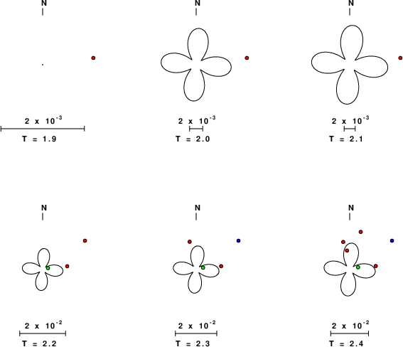
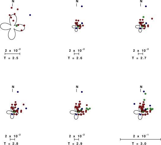
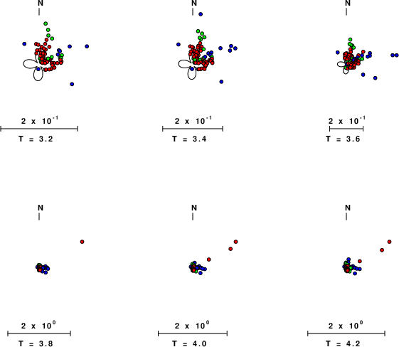
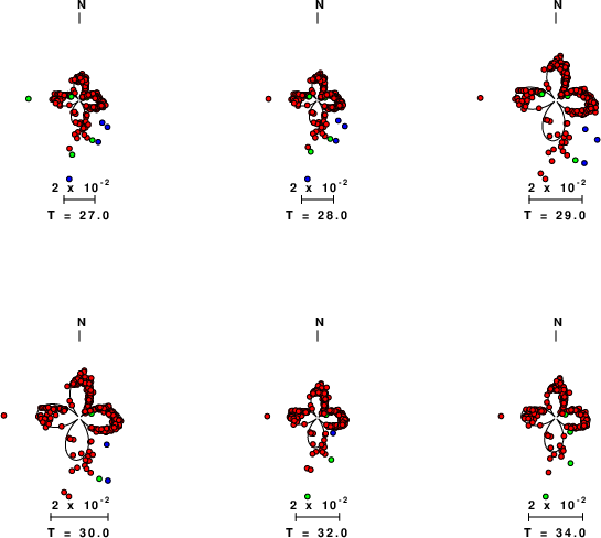
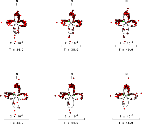
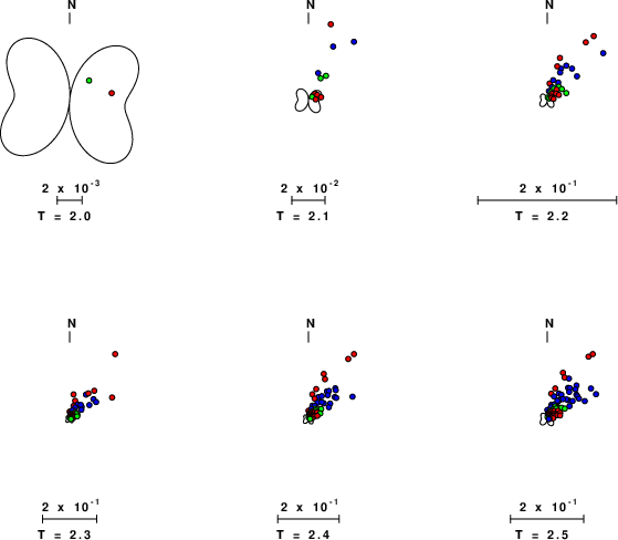
Love-wave radiation patterns
Rayleigh-wave radiation patterns