Left: mLg computed using the IASPEI formula. Center: mLg residuals versus epicentral distance ; the values used for the trimmed mean magnitude estimate are indicated. Right: residuals as a function of distance and azimuth.
The ANSS event ID is usp000jac0 and the event page is at https://earthquake.usgs.gov/earthquakes/eventpage/usp000jac0/executive.
2011/11/05 07:12:45 35.550 -96.764 3.1 4.8 Oklahoma
 USGS/SLU Moment Tensor Solution
 ENS  2011/11/05 07:12:45:0  35.55  -96.76   3.1 4.8 Oklahoma

 Stations used:
   AG.CCAR AG.FCAR AG.HHAR AG.LCAR AG.WHAR AG.WLAR IU.CCM
   NM.MGMO NM.PBMO NM.UALR TA.P34A TA.P35A TA.Q34A TA.Q35A
   TA.Q36A TA.Q37A TA.R34A TA.R35A TA.R36A TA.R37A TA.R38A
   TA.R39A TA.R40A TA.R41A TA.S34A TA.S35A TA.S36A TA.S37A
   TA.S38A TA.S39A TA.S40A TA.S41A TA.T34A TA.T35A TA.T36A
   TA.T37A TA.T38A TA.T39A TA.T40A TA.T41A TA.TUL1 TA.U35A
   TA.U36A TA.U37A TA.U38A TA.U39A TA.U41A TA.V35A TA.V36A
   TA.V37A TA.V38A TA.V39A TA.V40A TA.V41A TA.W35A TA.W36A
   TA.W37B TA.W38A TA.W39A TA.W40A TA.W41B TA.WHTX TA.X35A
   TA.X36A TA.X37A TA.X38A TA.Y35A TA.Y36A TA.Y37A TA.Y38A
   TA.Y39A TA.Z37A TA.Z38A US.CBKS US.KSU1 US.MIAR US.WMOK

 Filtering commands used:
   hp c 0.02 n 3
   lp c 0.07 n 3

 Best Fitting Double Couple
  Mo = 1.41e+23 dyne-cm
  Mw = 4.70
  Z  = 3 km
  Plane   Strike  Dip  Rake
   NP1       32    80   -170
   NP2      300    80   -10
  Principal Axes:
   Axis    Value   Plunge  Azimuth
    T   1.41e+23      0     166
    N   0.00e+00     76      75
    P  -1.41e+23     14     256

 Moment Tensor: (dyne-cm)
    Component   Value
       Mxx     1.25e+23
       Mxy    -6.49e+22
       Mxz     7.88e+21
       Myy    -1.17e+23
       Myz     3.24e+22
       Mzz    -8.39e+21


                     ##############
                 ######################
              ########################----
             #########################-----
           ##########################--------
          -#########################----------
         --------##################------------
        -------------##############-------------
        -----------------#########--------------
       ---------------------#####----------------
       ------------------------#-----------------
       -----------------------####---------------
       --   -----------------########------------
        - P ----------------############--------
        -   ---------------###############------
         ----------------###################---
          --------------######################
           ------------######################
             --------######################
              -----#######################
                 ###############   ####
                     ########### T


 Global CMT Convention Moment Tensor:
      R          T          P
 -8.39e+21   7.88e+21  -3.24e+22
  7.88e+21   1.25e+23   6.49e+22
 -3.24e+22   6.49e+22  -1.17e+23


Details of the solution is found at

http://www.eas.slu.edu/eqc/eqc_mt/MECH.NA/20111105071245/index.html
|
      STK = 300
      DIP = 80
     RAKE = -10
       MW = 4.70
       HS = 3.0
The NDK file is 20111105071245.ndk The waveform inversion is preferred.
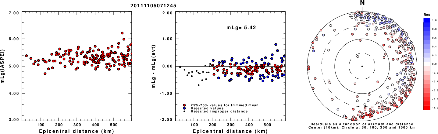
Given the availability of digital waveforms for determination of the moment tensor, this section documents the added processing leading to mLg, if appropriate to the region, and ML by application of the respective IASPEI formulae. As a research study, the linear distance term of the IASPEI formula for ML is adjusted to remove a linear distance trend in residuals to give a regionally defined ML. The defined ML uses horizontal component recordings, but the same procedure is applied to the vertical components since there may be some interest in vertical component ground motions. Residual plots versus distance may indicate interesting features of ground motion scaling in some distance ranges. A residual plot of the regionalized magnitude is given as a function of distance and azimuth, since data sets may transcend different wave propagation provinces.
Left: mLg computed using the IASPEI formula. Center: mLg residuals versus epicentral distance ; the values used for the trimmed mean magnitude estimate are indicated.
Right: residuals as a function of distance and azimuth.
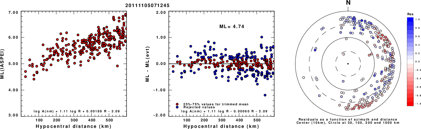
Left: ML computed using the IASPEI formula for Horizontal components. Center: ML residuals computed using a modified IASPEI formula that accounts for path specific attenuation; the values used for the trimmed mean are indicated. The ML relation used for each figure is given at the bottom of each plot.
Right: Residuals from new relation as a function of distance and azimuth.
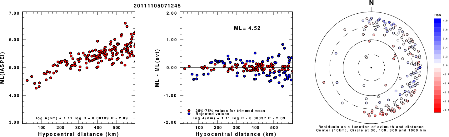
Left: ML computed using the IASPEI formula for Vertical components (research). Center: ML residuals computed using a modified IASPEI formula that accounts for path specific attenuation; the values used for the trimmed mean are indicated. The ML relation used for each figure is given at the bottom of each plot.
Right: Residuals from new relation as a function of distance and azimuth.
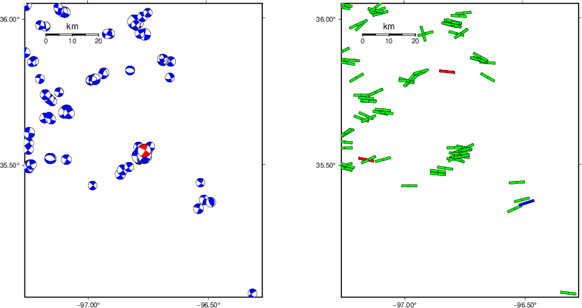 |
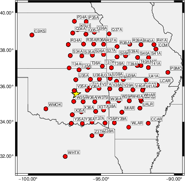
The focal mechanism was determined using broadband seismic waveforms. The location of the event (star) and the stations used for (red) the waveform inversion are shown in the next figure.
|
|
|
The program wvfgrd96 was used with good traces observed at short distance to determine the focal mechanism, depth and seismic moment. This technique requires a high quality signal and well determined velocity model for the Green's functions. To the extent that these are the quality data, this type of mechanism should be preferred over the radiation pattern technique which requires the separate step of defining the pressure and tension quadrants and the correct strike.
The observed and predicted traces are filtered using the following gsac commands:
hp c 0.02 n 3
lp c 0.07 n 3
The results of this grid search are as follow:
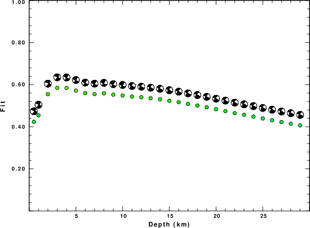
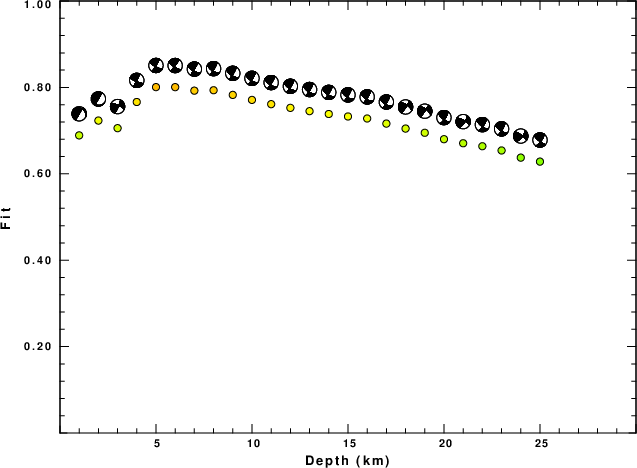
           DEPTH  STK   DIP  RAKE   MW    FIT
WVFGRD96    0.5   295    70   -20   4.52 0.4237
WVFGRD96    1.0   300    80   -10   4.54 0.4546
WVFGRD96    2.0   295    70   -20   4.67 0.5549
WVFGRD96    3.0   300    80   -10   4.70 0.5851
WVFGRD96    4.0   120    85     0   4.72 0.5844
WVFGRD96    5.0   120    80     0   4.75 0.5721
WVFGRD96    6.0   120    75     0   4.78 0.5599
WVFGRD96    7.0   120    70     0   4.80 0.5551
WVFGRD96    8.0   120    65     0   4.84 0.5587
WVFGRD96    9.0   120    65     0   4.85 0.5526
WVFGRD96   10.0   120    65     0   4.86 0.5486
WVFGRD96   11.0   120    90   -25   4.86 0.5437
WVFGRD96   12.0   120    90   -25   4.87 0.5405
WVFGRD96   13.0   120    90   -25   4.87 0.5359
WVFGRD96   14.0   120    90   -25   4.88 0.5304
WVFGRD96   15.0   120    90   -25   4.89 0.5238
WVFGRD96   16.0   120    90   -25   4.90 0.5168
WVFGRD96   17.0   300    90    25   4.91 0.5088
WVFGRD96   18.0   120    90   -25   4.92 0.5009
WVFGRD96   19.0   120    90   -25   4.92 0.4925
WVFGRD96   20.0   120    90   -25   4.93 0.4834
WVFGRD96   21.0   120    90   -25   4.94 0.4744
WVFGRD96   22.0   120    90   -25   4.95 0.4648
WVFGRD96   23.0   300    85    25   4.95 0.4568
WVFGRD96   24.0   300    85    25   4.96 0.4482
WVFGRD96   25.0   300    85    25   4.96 0.4395
WVFGRD96   26.0   300    85    25   4.97 0.4311
WVFGRD96   27.0   300    85    25   4.97 0.4226
WVFGRD96   28.0   300    85    25   4.98 0.4146
WVFGRD96   29.0   300    85    25   4.99 0.4066
The best solution is
WVFGRD96 3.0 300 80 -10 4.70 0.5851
The mechanism corresponding to the best fit is
|
|
|
The best fit as a function of depth is given in the following figure:
|
|
|
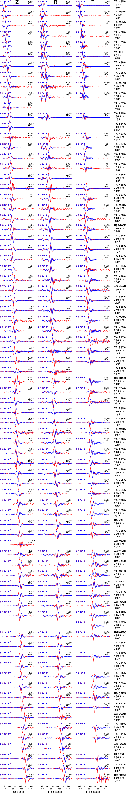
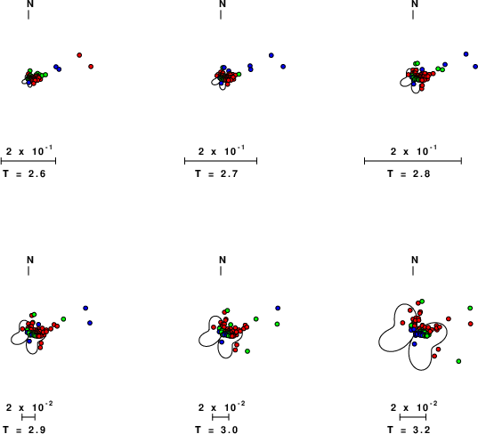
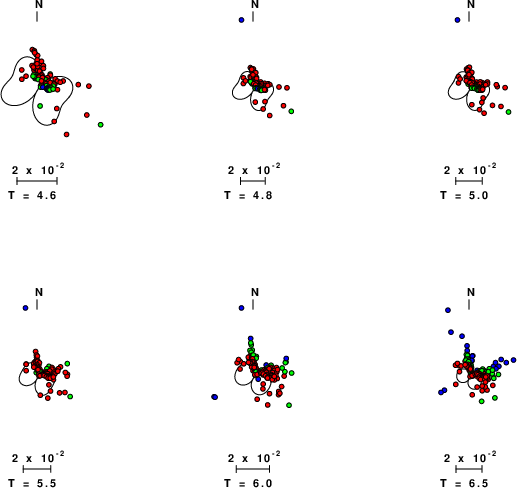
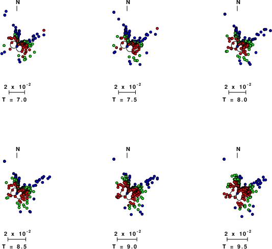
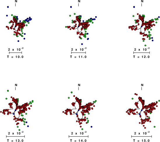
The comparison of the observed and predicted waveforms is given in the next figure. The red traces are the observed and the blue are the predicted. Each observed-predicted component is plotted to the same scale and peak amplitudes are indicated by the numbers to the left of each trace. A pair of numbers is given in black at the right of each predicted traces. The upper number it the time shift required for maximum correlation between the observed and predicted traces. This time shift is required because the synthetics are not computed at exactly the same distance as the observed, the velocity model used in the predictions may not be perfect and the epicentral parameters may be be off. A positive time shift indicates that the prediction is too fast and should be delayed to match the observed trace (shift to the right in this figure). A negative value indicates that the prediction is too slow. The lower number gives the percentage of variance reduction to characterize the individual goodness of fit (100% indicates a perfect fit).
The bandpass filter used in the processing and for the display was
hp c 0.02 n 3
lp c 0.07 n 3
|
| Figure 3. Waveform comparison for selected depth. Red: observed; Blue - predicted. The time shift with respect to the model prediction is indicated. The percent of fit is also indicated. The time scale is relative to the first trace sample. |
|
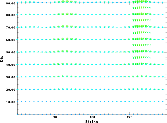
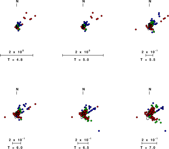
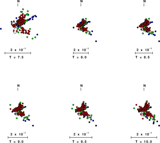
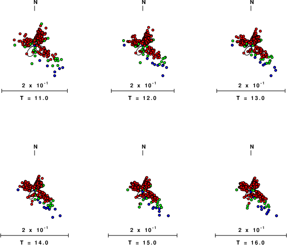
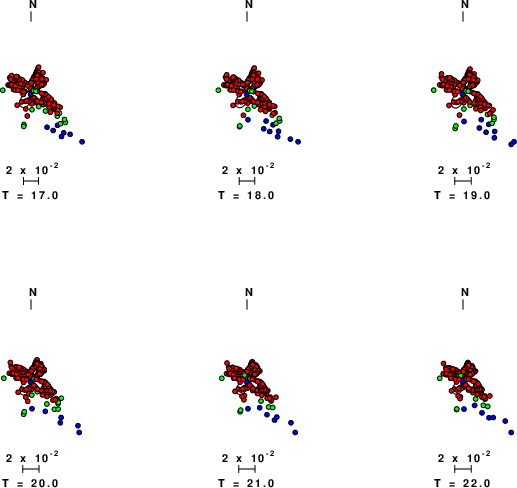
| Focal mechanism sensitivity at the preferred depth. The red color indicates a very good fit to the waveforms. Each solution is plotted as a vector at a given value of strike and dip with the angle of the vector representing the rake angle, measured, with respect to the upward vertical (N) in the figure. |
A check on the assumed source location is possible by looking at the time shifts between the observed and predicted traces. The time shifts for waveform matching arise for several reasons:
Time_shift = A + B cos Azimuth + C Sin Azimuth
The time shifts for this inversion lead to the next figure:
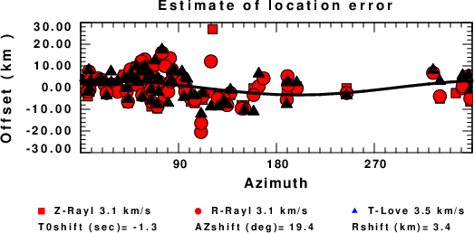
The derived shift in origin time and epicentral coordinates are given at the bottom of the figure.
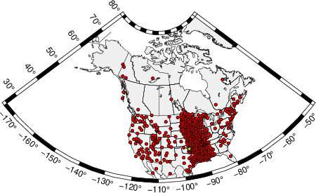
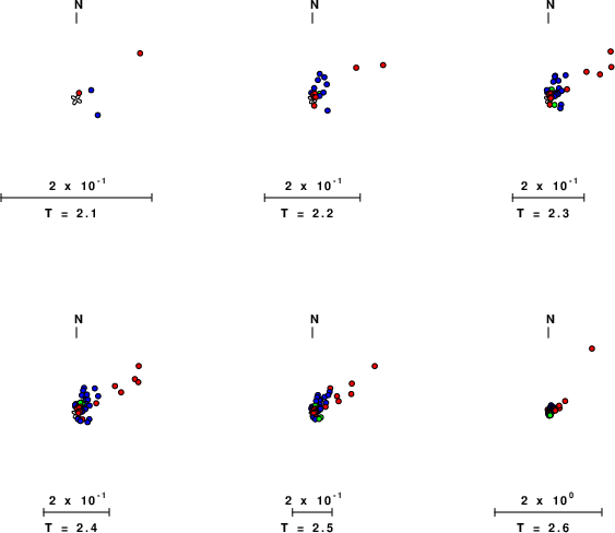
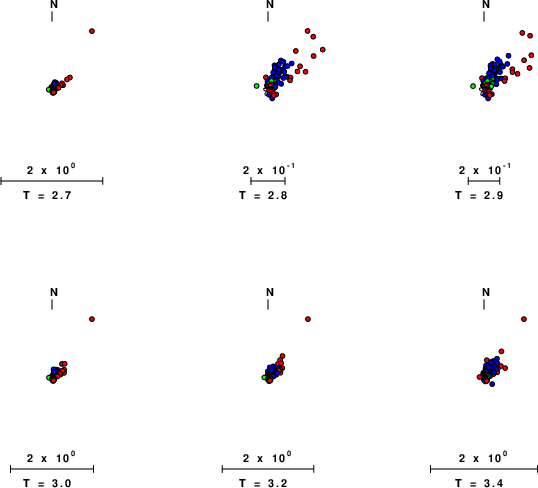
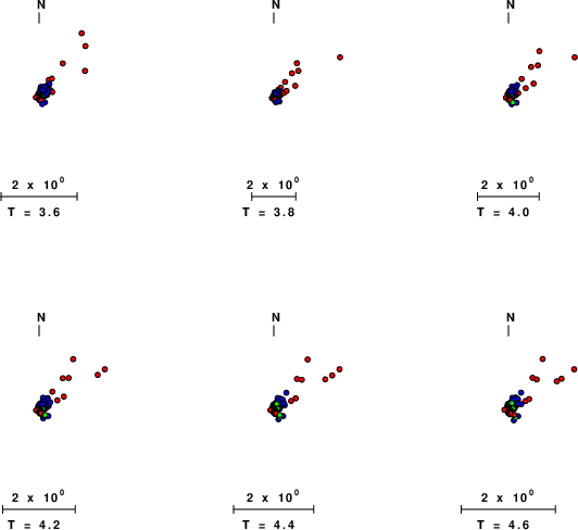
The following figure shows the stations used in the grid search for the best focal mechanism to fit the surface-wave spectral amplitudes of the Love and Rayleigh waves.
|
|
|
The surface-wave determined focal mechanism is shown here.
  NODAL PLANES


  STK=      29.99
  DIP=      90.00
 RAKE=    -165.00

             OR

  STK=     299.99
  DIP=      75.00
 RAKE=       0.00


DEPTH = 5.0 km

Mw = 4.93
Best Fit 0.8008 - P-T axis plot gives solutions with FIT greater than FIT90
 |
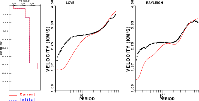
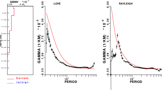
Surface wave analysis was performed using codes from Computer Programs in Seismology, specifically the multiple filter analysis program do_mft and the surface-wave radiation pattern search program srfgrd96.
Digital data were collected, instrument response removed and traces converted
to Z, R an T components. Multiple filter analysis was applied to the Z and T traces to obtain the Rayleigh- and Love-wave spectral amplitudes, respectively.
These were input to the search program which examined all depths between 1 and 25 km
and all possible mechanisms.
|
|
|
|
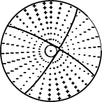
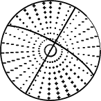
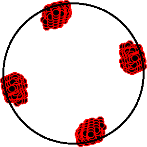
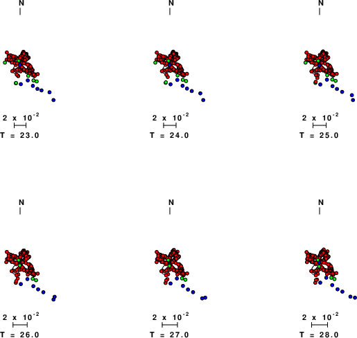
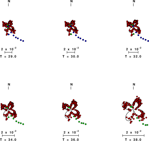
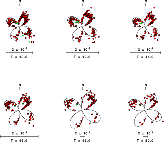
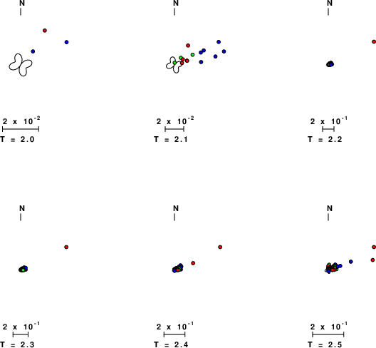
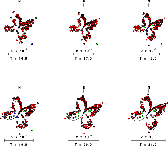
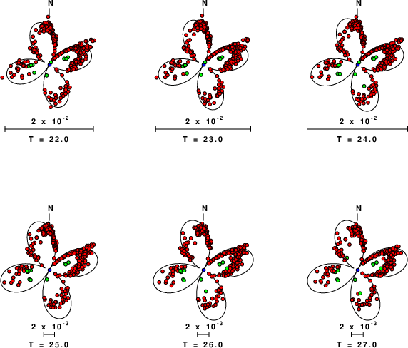
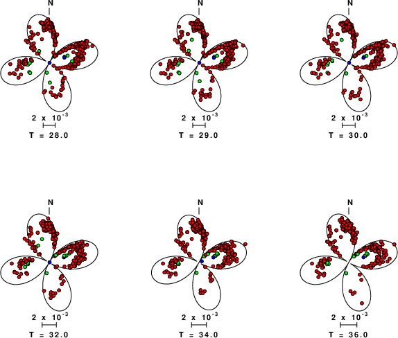
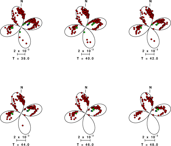
| Pressure-tension axis trends. Since the surface-wave spectra search does not distinguish between P and T axes and since there is a 180 ambiguity in strike, all possible P and T axes are plotted. First motion data and waveforms will be used to select the preferred mechanism. The purpose of this plot is to provide an idea of the possible range of solutions. The P and T-axes for all mechanisms with goodness of fit greater than 0.9 FITMAX (above) are plotted here. |
|
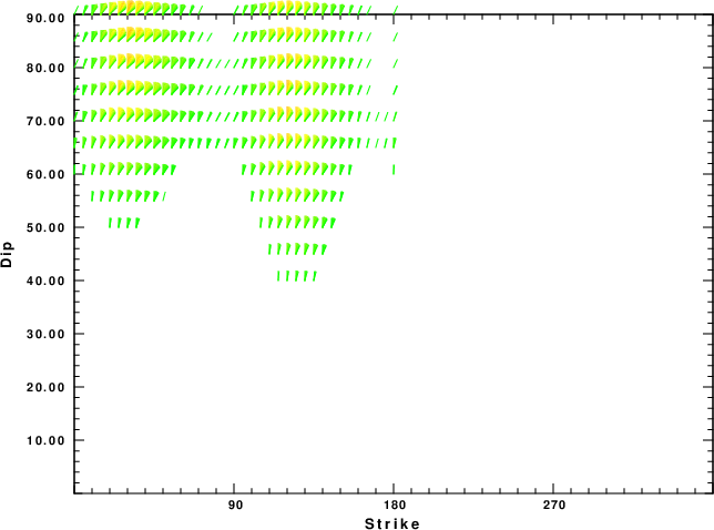
| Focal mechanism sensitivity at the preferred depth. The red color indicates a very good fit to the Love and Rayleigh wave radiation patterns. Each solution is plotted as a vector at a given value of strike and dip with the angle of the vector representing the rake angle, measured, with respect to the upward vertical (N) in the figure. Because of the symmetry of the spectral amplitude rediation patterns, only strikes from 0-180 degrees are sampled. |
|
|
The WUS.model used for the waveform synthetic seismograms and for the surface wave eigenfunctions and dispersion is as follows (The format is in the model96 format of Computer Programs in Seismology).
MODEL.01
Model after     8 iterations
ISOTROPIC
KGS
FLAT EARTH
1-D
CONSTANT VELOCITY
LINE08
LINE09
LINE10
LINE11
      H(KM)   VP(KM/S)   VS(KM/S) RHO(GM/CC)         QP         QS       ETAP       ETAS      FREFP      FREFS
     1.9000     3.4065     2.0089     2.2150  0.302E-02  0.679E-02   0.00       0.00       1.00       1.00
     6.1000     5.5445     3.2953     2.6089  0.349E-02  0.784E-02   0.00       0.00       1.00       1.00
    13.0000     6.2708     3.7396     2.7812  0.212E-02  0.476E-02   0.00       0.00       1.00       1.00
    19.0000     6.4075     3.7680     2.8223  0.111E-02  0.249E-02   0.00       0.00       1.00       1.00
     0.0000     7.9000     4.6200     3.2760  0.164E-10  0.370E-10   0.00       0.00       1.00       1.00