Location
SLU Location
To check the ANSS location or to compare the observed P-wave first motions to the moment tensor solution, P- and S-wave first arrival times were manually read together with the P-wave first motions. The subsequent output of the program elocate is given in the file elocate.txt. The first motion plot is shown below.
Location ANSS
The ANSS event ID is usp000j8jr and the event page is at
https://earthquake.usgs.gov/earthquakes/eventpage/usp000j8jr/executive.
2011/09/26 01:02:53 63.434 -126.278 1.0 5.3 NWT, Canada
Focal Mechanism
 USGS/SLU Moment Tensor Solution
 ENS  2011/09/26 01:02:53:0  63.43 -126.28   1.0 5.3 NWT, Canada

 Stations used:
   AK.BESE AK.BMR AK.DCPH AK.DOT AK.FYU AK.TGL AT.CRAG AT.YKU2
   CN.BVCY CN.CLVN CN.DAWY CN.DHRN CN.DLBC CN.FNBB CN.HPLN
   CN.INK CN.KUKN CN.PLBC CN.SMPN CN.WHFN CN.WHY CN.YKW3
   CN.YUK1 CN.YUK2 CN.YUK3 US.EGAK US.WRAK

 Filtering commands used:
   hp c 0.01 n 3
   lp c 0.03 n 3

 Best Fitting Double Couple
  Mo = 4.57e+23 dyne-cm
  Mw = 5.04
  Z  = 3 km
  Plane   Strike  Dip  Rake
   NP1      320    60    90
   NP2      140    30    90
  Principal Axes:
   Axis    Value   Plunge  Azimuth
    T   4.57e+23     75     230
    N   0.00e+00     -0     140
    P  -4.57e+23     15      50

 Moment Tensor: (dyne-cm)
    Component   Value
       Mxx    -1.64e+23
       Mxy    -1.95e+23
       Mxz    -1.47e+23
       Myy    -2.32e+23
       Myz    -1.75e+23
       Mzz     3.96e+23


                     --------------
                 ----------------------
              -##-------------------------
             ##########-----------------
           --#############-------------- P --
          --################------------   ---
         ---###################----------------
        ---#####################----------------
        ---#######################--------------
       -----#######################--------------
       -----#########################------------
       -----###########   ############-----------
       ------########## T #############----------
        ------#########   ##############--------
        -------#########################--------
         -------#########################------
          -------########################-----
           --------######################----
             ---------####################-
              -----------################-
                 ----------------------
                     --------------


 Global CMT Convention Moment Tensor:
      R          T          P
  3.96e+23  -1.47e+23   1.75e+23
 -1.47e+23  -1.64e+23   1.95e+23
  1.75e+23   1.95e+23  -2.32e+23


Details of the solution is found at

http://www.eas.slu.edu/eqc/eqc_mt/MECH.NA/20110926010253/index.html
|
Preferred Solution
The preferred solution from an analysis of the surface-wave spectral amplitude radiation pattern, waveform inversion or first motion observations is
      STK = 140
      DIP = 30
     RAKE = 90
       MW = 5.04
       HS = 3.0
The NDK file is 20110926010253.ndk
The waveform inversion is preferred.
Moment Tensor Comparison
The following compares this source inversion to those provided by others. The purpose is to look for major differences and also to note slight differences that might be inherent to the processing procedure. For completeness the USGS/SLU solution is repeated from above.
| SLU |
SLUFM |
 USGS/SLU Moment Tensor Solution
 ENS  2011/09/26 01:02:53:0  63.43 -126.28   1.0 5.3 NWT, Canada

 Stations used:
   AK.BESE AK.BMR AK.DCPH AK.DOT AK.FYU AK.TGL AT.CRAG AT.YKU2
   CN.BVCY CN.CLVN CN.DAWY CN.DHRN CN.DLBC CN.FNBB CN.HPLN
   CN.INK CN.KUKN CN.PLBC CN.SMPN CN.WHFN CN.WHY CN.YKW3
   CN.YUK1 CN.YUK2 CN.YUK3 US.EGAK US.WRAK

 Filtering commands used:
   hp c 0.01 n 3
   lp c 0.03 n 3

 Best Fitting Double Couple
  Mo = 4.57e+23 dyne-cm
  Mw = 5.04
  Z  = 3 km
  Plane   Strike  Dip  Rake
   NP1      320    60    90
   NP2      140    30    90
  Principal Axes:
   Axis    Value   Plunge  Azimuth
    T   4.57e+23     75     230
    N   0.00e+00     -0     140
    P  -4.57e+23     15      50

 Moment Tensor: (dyne-cm)
    Component   Value
       Mxx    -1.64e+23
       Mxy    -1.95e+23
       Mxz    -1.47e+23
       Myy    -2.32e+23
       Myz    -1.75e+23
       Mzz     3.96e+23


                     --------------
                 ----------------------
              -##-------------------------
             ##########-----------------
           --#############-------------- P --
          --################------------   ---
         ---###################----------------
        ---#####################----------------
        ---#######################--------------
       -----#######################--------------
       -----#########################------------
       -----###########   ############-----------
       ------########## T #############----------
        ------#########   ##############--------
        -------#########################--------
         -------#########################------
          -------########################-----
           --------######################----
             ---------####################-
              -----------################-
                 ----------------------
                     --------------


 Global CMT Convention Moment Tensor:
      R          T          P
  3.96e+23  -1.47e+23   1.75e+23
 -1.47e+23  -1.64e+23   1.95e+23
  1.75e+23   1.95e+23  -2.32e+23


Details of the solution is found at

http://www.eas.slu.edu/eqc/eqc_mt/MECH.NA/20110926010253/index.html
|
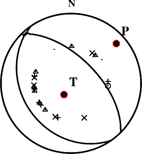
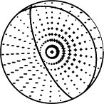
First motions and takeoff angles from an elocate run.
|
Magnitudes
Given the availability of digital waveforms for determination of the moment tensor, this section documents the added processing leading to mLg, if appropriate to the region, and ML by application of the respective IASPEI formulae. As a research study, the linear distance term of the IASPEI formula
for ML is adjusted to remove a linear distance trend in residuals to give a regionally defined ML. The defined ML uses horizontal component recordings, but the same procedure is applied to the vertical components since there may be some interest in vertical component ground motions. Residual plots versus distance may indicate interesting features of ground motion scaling in some distance ranges. A residual plot of the regionalized magnitude is given as a function of distance and azimuth, since data sets may transcend different wave propagation provinces.
Context
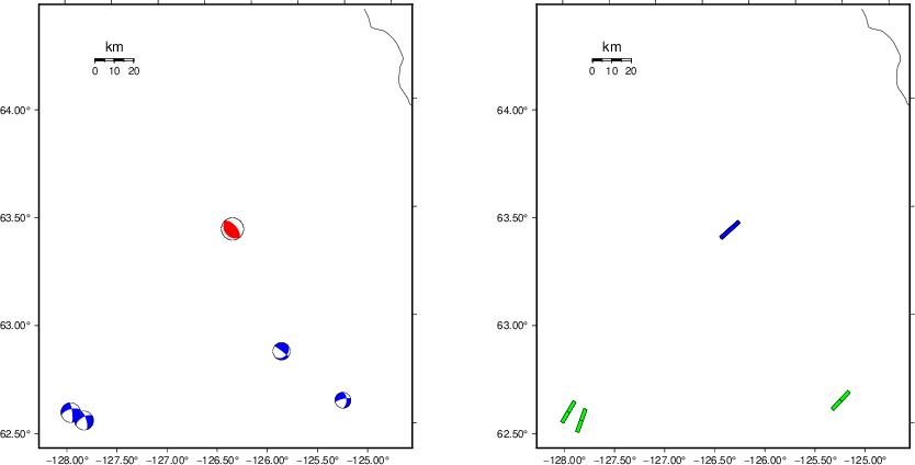
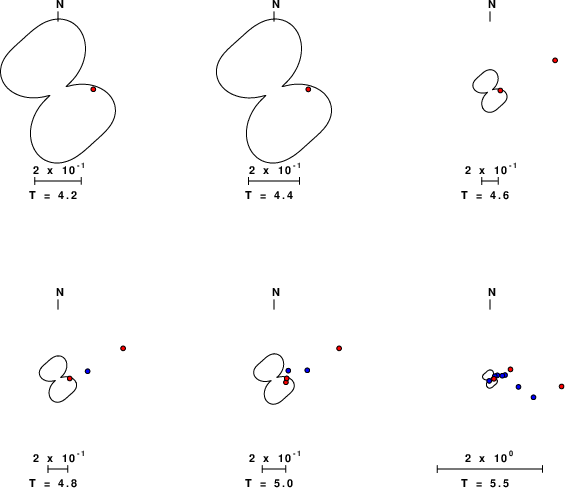
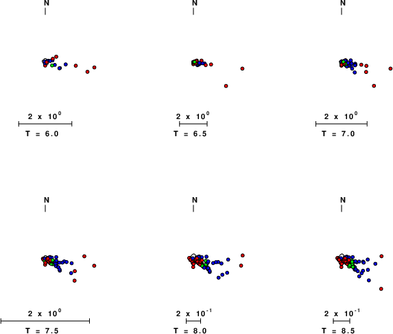
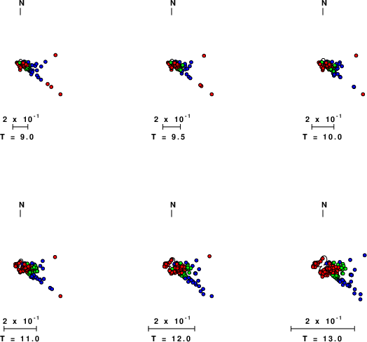
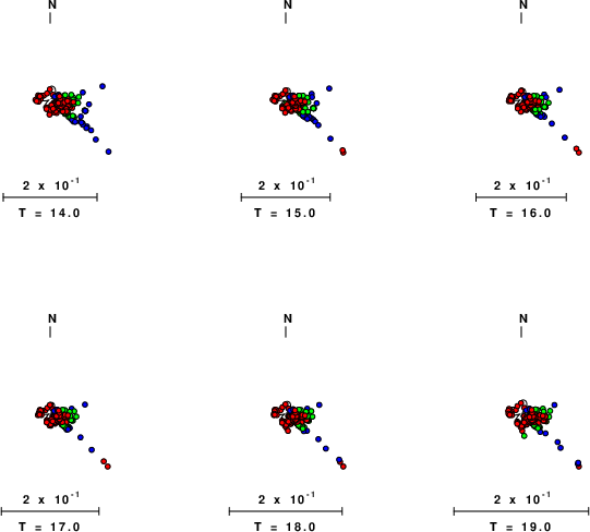
The left panel of the next figure presents the focal mechanism for this earthquake (red) in the context of other nearby events (blue) in the SLU Moment Tensor Catalog. The right panel shows the inferred direction of maximum compressive stress and the type of faulting (green is strike-slip, red is normal, blue is thrust; oblique is shown by a combination of colors). Thus context plot is useful for assessing the appropriateness of the moment tensor of this event.
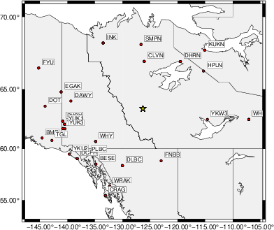
Waveform Inversion using wvfgrd96
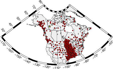
The focal mechanism was determined using broadband seismic waveforms. The location of the event (star) and the
stations used for (red) the waveform inversion are shown in the next figure.
|
|
Location of broadband stations used for waveform inversion
|
The program wvfgrd96 was used with good traces observed at short distance to determine the focal mechanism, depth and seismic moment. This technique requires a high quality signal and well determined velocity model for the Green's functions. To the extent that these are the quality data, this type of mechanism should be preferred over the radiation pattern technique which requires the separate step of defining the pressure and tension quadrants and the correct strike.
The observed and predicted traces are filtered using the following gsac commands:
hp c 0.01 n 3
lp c 0.03 n 3
The results of this grid search are as follow:
           DEPTH  STK   DIP  RAKE   MW    FIT
WVFGRD96    0.5   305    70    80   5.01 0.5439
WVFGRD96    1.0   315    55    85   4.94 0.5597
WVFGRD96    2.0   140    30    90   4.99 0.5728
WVFGRD96    3.0   140    30    90   5.04 0.5743
WVFGRD96    4.0   140    30    90   5.06 0.5568
WVFGRD96    5.0   140    25    90   5.11 0.5340
WVFGRD96    6.0   140    25    90   5.11 0.5120
WVFGRD96    7.0   320    65    90   5.11 0.4918
WVFGRD96    8.0   135    25    85   5.15 0.4988
WVFGRD96    9.0   140    75    90   5.16 0.4963
WVFGRD96   10.0   315    15    85   5.15 0.5133
WVFGRD96   11.0   315    15    85   5.14 0.5261
WVFGRD96   12.0   315    15    85   5.13 0.5357
WVFGRD96   13.0   310    15    80   5.13 0.5420
WVFGRD96   14.0   310    15    80   5.12 0.5464
WVFGRD96   15.0   310    15    80   5.11 0.5489
WVFGRD96   16.0   305    15    75   5.11 0.5497
WVFGRD96   17.0   295    15    60   5.10 0.5495
WVFGRD96   18.0   295    15    60   5.10 0.5482
WVFGRD96   19.0   295    15    60   5.09 0.5466
WVFGRD96   20.0   290    15    55   5.09 0.5445
WVFGRD96   21.0   290    15    55   5.10 0.5434
WVFGRD96   22.0   285    15    50   5.09 0.5405
WVFGRD96   23.0   280    15    45   5.09 0.5368
WVFGRD96   24.0   285    15    50   5.09 0.5329
WVFGRD96   25.0   270    20    30   5.09 0.5293
WVFGRD96   26.0   270    20    30   5.09 0.5249
WVFGRD96   27.0   270    20    30   5.09 0.5210
WVFGRD96   28.0   270    20    30   5.09 0.5165
WVFGRD96   29.0   270    20    30   5.09 0.5114
The best solution is
WVFGRD96 3.0 140 30 90 5.04 0.5743
The mechanism corresponding to the best fit is
|
|
Figure 1. Waveform inversion focal mechanism
|
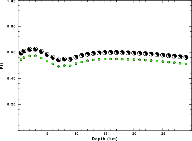
The best fit as a function of depth is given in the following figure:
|
|
Figure 2. Depth sensitivity for waveform mechanism
|
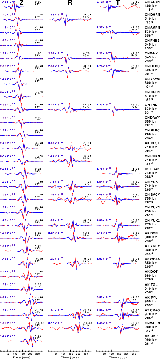
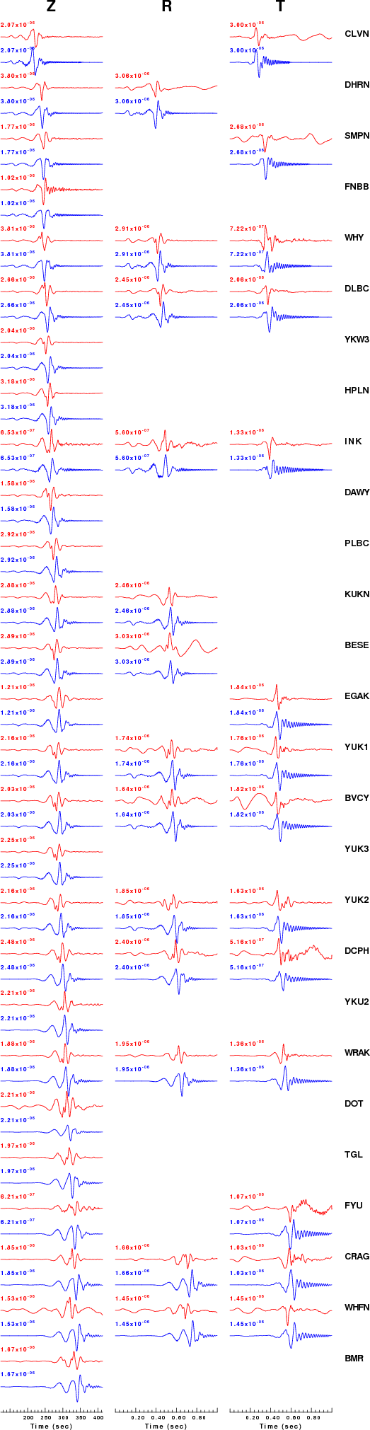
The comparison of the observed and predicted waveforms is given in the next figure. The red traces are the observed and the blue are the predicted.
Each observed-predicted component is plotted to the same scale and peak amplitudes are indicated by the numbers to the left of each trace. A pair of numbers is given in black at the right of each predicted traces. The upper number it the time shift required for maximum correlation between the observed and predicted traces. This time shift is required because the synthetics are not computed at exactly the same distance as the observed, the velocity model used in the predictions may not be perfect and the epicentral parameters may be be off.
A positive time shift indicates that the prediction is too fast and should be delayed to match the observed trace (shift to the right in this figure). A negative value indicates that the prediction is too slow. The lower number gives the percentage of variance reduction to characterize the individual goodness of fit (100% indicates a perfect fit).
The bandpass filter used in the processing and for the display was
hp c 0.01 n 3
lp c 0.03 n 3
|
|
Figure 3. Waveform comparison for selected depth. Red: observed; Blue - predicted. The time shift with respect to the model prediction is indicated. The percent of fit is also indicated. The time scale is relative to the first trace sample.
|
|
|
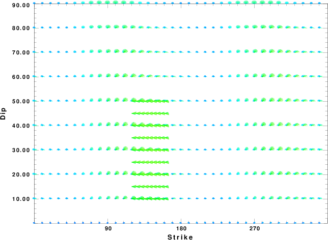
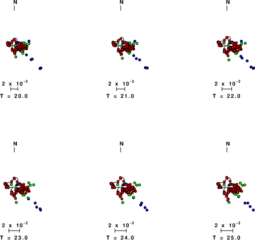
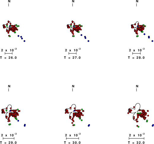
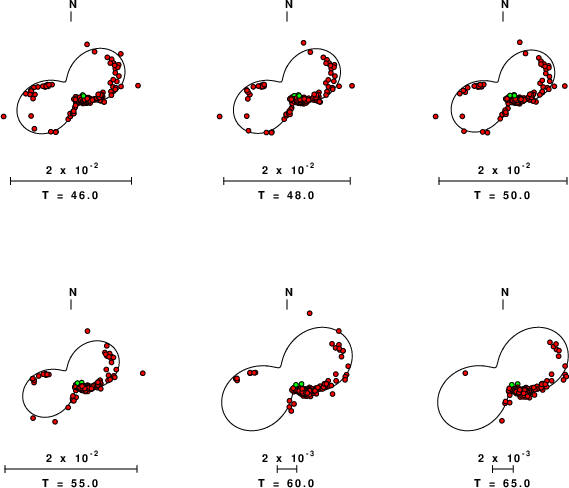
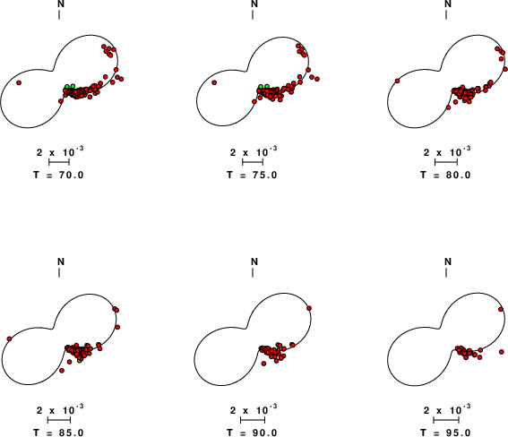
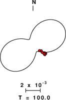
Focal mechanism sensitivity at the preferred depth. The red color indicates a very good fit to the waveforms.
Each solution is plotted as a vector at a given value of strike and dip with the angle of the vector representing the rake angle, measured, with respect to the upward vertical (N) in the figure.
|
A check on the assumed source location is possible by looking at the time shifts between the observed and predicted traces. The time shifts for waveform matching arise for several reasons:
- The origin time and epicentral distance are incorrect
- The velocity model used for the inversion is incorrect
- The velocity model used to define the P-arrival time is not the
same as the velocity model used for the waveform inversion
(assuming that the initial trace alignment is based on the
P arrival time)
Assuming only a mislocation, the time shifts are fit to a functional form:
Time_shift = A + B cos Azimuth + C Sin Azimuth
The time shifts for this inversion lead to the next figure:
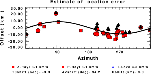
The derived shift in origin time and epicentral coordinates are given at the bottom of the figure.
Surface-Wave Focal Mechanism
The following figure shows the stations used in the grid search for the best focal mechanism to fit the surface-wave spectral amplitudes of the Love and Rayleigh waves.
|
|
Location of broadband stations used to obtain focal mechanism from surface-wave spectral amplitudes
|
The surface-wave determined focal mechanism is shown here.
  NODAL PLANES


  STK=     155.90
  DIP=      70.71
 RAKE=      95.39

             OR

  STK=     319.97
  DIP=      20.00
 RAKE=      74.98


DEPTH = 1.0 km

Mw = 5.16
Best Fit 0.8061 - P-T axis plot gives solutions with FIT greater than FIT90
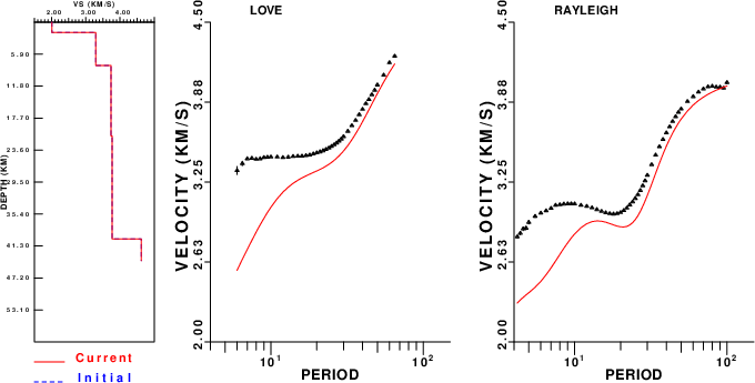
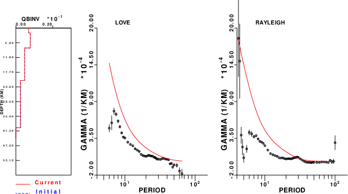
Surface-wave analysis
Surface wave analysis was performed using codes from
Computer Programs in Seismology, specifically the
multiple filter analysis program do_mft and the surface-wave
radiation pattern search program srfgrd96.
Data preparation
Digital data were collected, instrument response removed and traces converted
to Z, R an T components. Multiple filter analysis was applied to the Z and T traces to obtain the Rayleigh- and Love-wave spectral amplitudes, respectively.
These were input to the search program which examined all depths between 1 and 25 km
and all possible mechanisms.
|
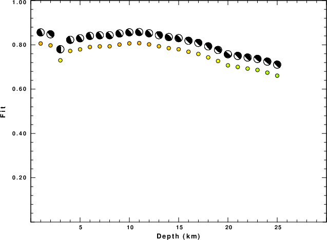
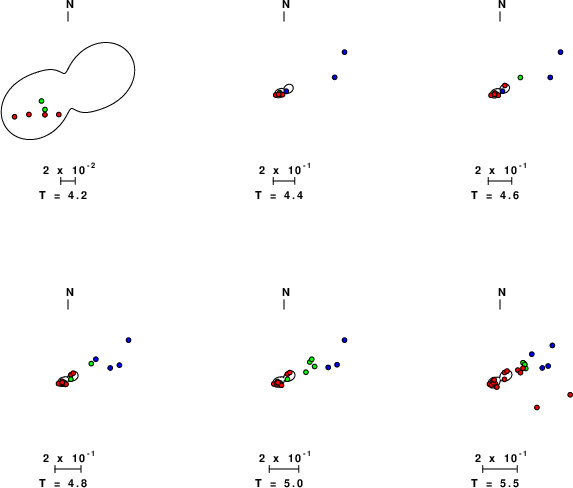
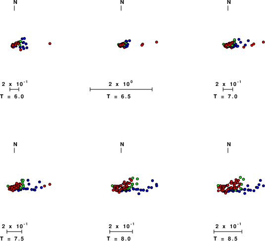
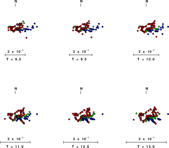
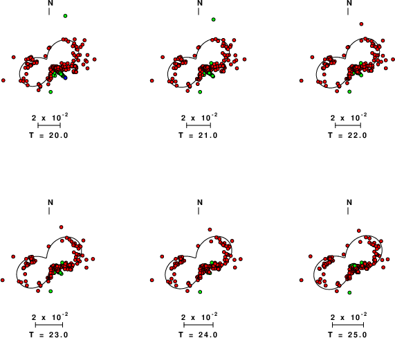
|
Best mechanism fit as a function of depth. The preferred depth is given above. Lower hemisphere projection
|
|
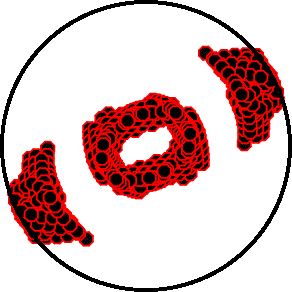
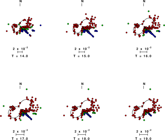
|
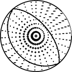
Pressure-tension axis trends. Since the surface-wave spectra search does not distinguish between P and T axes and since there is a 180 ambiguity in strike, all possible P and T axes are plotted. First motion data and waveforms will be used to select the preferred mechanism. The purpose of this plot is to provide an idea of the
possible range of solutions. The P and T-axes for all mechanisms with goodness of fit greater than 0.9 FITMAX (above) are plotted here.
|
|
|
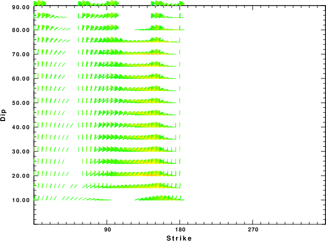
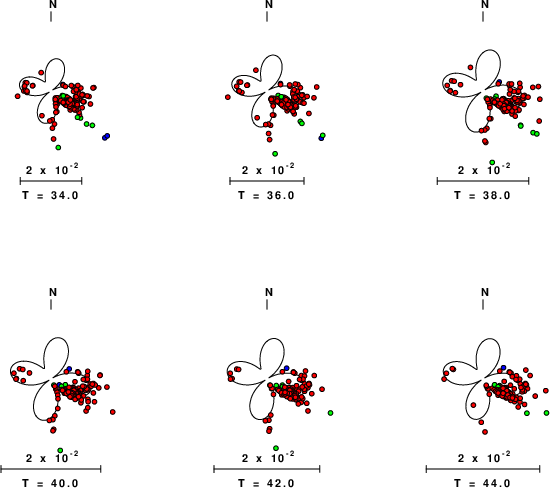
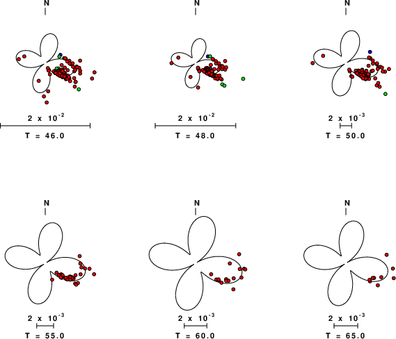
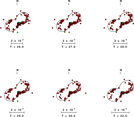
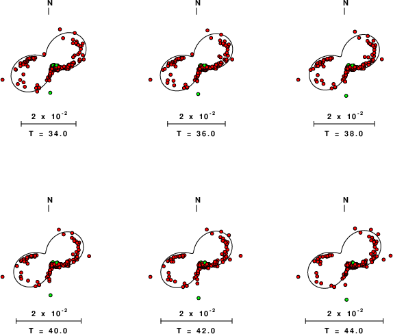
Focal mechanism sensitivity at the preferred depth. The red color indicates a very good fit to the Love and Rayleigh wave radiation patterns.
Each solution is plotted as a vector at a given value of strike and dip with the angle of the vector representing the rake angle, measured, with respect to the upward vertical (N) in the figure. Because of the symmetry of the spectral amplitude rediation patterns, only strikes from 0-180 degrees are sampled.
|
Love-wave radiation patterns
Rayleigh-wave radiation patterns
- Rayleigh-wave radiation patterns.
- Rayleigh-wave radiation patterns.
- Rayleigh-wave radiation patterns.
- Rayleigh-wave radiation patterns.
- Rayleigh-wave radiation patterns.
- Rayleigh-wave radiation patterns.
- Rayleigh-wave radiation patterns.
- Rayleigh-wave radiation patterns.
- Rayleigh-wave radiation patterns.
- Rayleigh-wave radiation patterns.
Waveform comparison for this mechanism
Since the analysis of the surface-wave radiation patterns uses only spectral
amplitudes and because the surfave-wave radiation patterns have a 180 degree symmetry, each surface-wave solution consists of four possible focal mechanisms corresponding to the interchange of the P- and T-axes and a roation of the mechanism by 180 degrees. To select one mechanism, P-wave first motion can be used. This was not possible in this case because all the P-wave first motions were
emergent ( a feature of the P-wave wave takeoff angle, the station location and the mechanism). The other way to select among the mechanisms is to compute
forward synthetics and compare the observed and predicted waveforms.
The fits to the waveforms with the given mechanism are show below:
This figure shows the fit to the three components of motion (Z - vertical, R-radial and T - transverse). For each station and component, the
observed traces is shown in red and the model predicted trace in blue. The traces represent filtered ground velocity in units of meters/sec (the peak value is printed adjacent to each trace; each pair of traces to plotted to the same scale to emphasize the difference in levels). Both synthetic and observed traces have been filtered using the SAC commands:
Appendix A
Spectra fit plots to each station
Velocity Model
The WUS.model used for the waveform synthetic seismograms and for the surface wave eigenfunctions and dispersion is as follows
(The format is in the model96 format of Computer Programs in Seismology).
MODEL.01
Model after     8 iterations
ISOTROPIC
KGS
FLAT EARTH
1-D
CONSTANT VELOCITY
LINE08
LINE09
LINE10
LINE11
      H(KM)   VP(KM/S)   VS(KM/S) RHO(GM/CC)         QP         QS       ETAP       ETAS      FREFP      FREFS
     1.9000     3.4065     2.0089     2.2150  0.302E-02  0.679E-02   0.00       0.00       1.00       1.00
     6.1000     5.5445     3.2953     2.6089  0.349E-02  0.784E-02   0.00       0.00       1.00       1.00
    13.0000     6.2708     3.7396     2.7812  0.212E-02  0.476E-02   0.00       0.00       1.00       1.00
    19.0000     6.4075     3.7680     2.8223  0.111E-02  0.249E-02   0.00       0.00       1.00       1.00
     0.0000     7.9000     4.6200     3.2760  0.164E-10  0.370E-10   0.00       0.00       1.00       1.00
Last Changed Sat Apr 27 04:33:06 PM CDT 2024