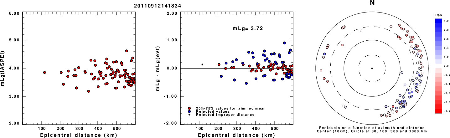
Left: mLg computed using the IASPEI formula. Center: mLg residuals versus epicentral distance ; the values used for the trimmed mean magnitude estimate are indicated. Right: residuals as a function of distance and azimuth.
The ANSS event ID is usp000j7yp and the event page is at https://earthquake.usgs.gov/earthquakes/eventpage/usp000j7yp/executive.
2011/09/12 14:18:34 32.822 -100.871 7.9 4.30 Texas
 USGS/SLU Moment Tensor Solution
 ENS  2011/09/12 14:18:34:6  32.82 -100.87   7.9 4.3 Texas

 Stations used:
   TA.233A TA.234A TA.236A TA.333A TA.334A TA.335A TA.435B
   TA.436A TA.534A TA.633A TA.634A TA.ABTX TA.MSTX TA.W35A
   TA.WHTX TA.X35A TA.Y36A TA.Z36A US.MNTX US.WMOK

 Filtering commands used:
   cut o DIST/3.3 -40 o DIST/3.3 +50
   rtr
   taper w 0.1
   hp c 0.03 n 3
   lp c 0.10 n 3
   br c 0.12 0.25 n 4 p 2

 Best Fitting Double Couple
  Mo = 2.85e+21 dyne-cm
  Mw = 3.57
  Z  = 10 km
  Plane   Strike  Dip  Rake
   NP1      300    70    30
   NP2      199    62   157
  Principal Axes:
   Axis    Value   Plunge  Azimuth
    T   2.85e+21     35     162
    N   0.00e+00     54     331
    P  -2.85e+21      5      68

 Moment Tensor: (dyne-cm)
    Component   Value
       Mxx     1.32e+21
       Mxy    -1.56e+21
       Mxz    -1.37e+21
       Myy    -2.24e+21
       Myz     1.85e+20
       Mzz     9.16e+20


                     #############-
                 ##############--------
              ###############-------------
             ###############---------------
           ###############-------------------
          -----##########---------------------
         -------------##---------------------
        ---------------####------------------ P
        --------------########---------------
       --------------############----------------
       --------------###############-------------
       -------------##################-----------
       -------------####################---------
        ------------######################------
        -----------#########################----
         ----------##########################--
          ---------###########################
           --------############   ###########
             ------############ T #########
              ------###########   ########
                 ---###################
                     ##############


 Global CMT Convention Moment Tensor:
      R          T          P
  9.16e+20  -1.37e+21  -1.85e+20
 -1.37e+21   1.32e+21   1.56e+21
 -1.85e+20   1.56e+21  -2.24e+21


Details of the solution is found at

http://www.eas.slu.edu/eqc/eqc_mt/MECH.NA/20110912141834/index.html
|
      STK = 300
      DIP = 70
     RAKE = 30
       MW = 3.57
       HS = 10.0
The NDK file is 20110912141834.ndk The waveform inversion is preferred.
Given the availability of digital waveforms for determination of the moment tensor, this section documents the added processing leading to mLg, if appropriate to the region, and ML by application of the respective IASPEI formulae. As a research study, the linear distance term of the IASPEI formula for ML is adjusted to remove a linear distance trend in residuals to give a regionally defined ML. The defined ML uses horizontal component recordings, but the same procedure is applied to the vertical components since there may be some interest in vertical component ground motions. Residual plots versus distance may indicate interesting features of ground motion scaling in some distance ranges. A residual plot of the regionalized magnitude is given as a function of distance and azimuth, since data sets may transcend different wave propagation provinces.
Left: mLg computed using the IASPEI formula. Center: mLg residuals versus epicentral distance ; the values used for the trimmed mean magnitude estimate are indicated.
Right: residuals as a function of distance and azimuth.
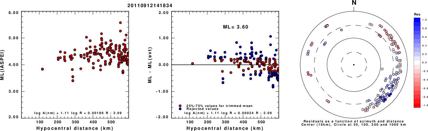
Left: ML computed using the IASPEI formula for Horizontal components. Center: ML residuals computed using a modified IASPEI formula that accounts for path specific attenuation; the values used for the trimmed mean are indicated. The ML relation used for each figure is given at the bottom of each plot.
Right: Residuals from new relation as a function of distance and azimuth.
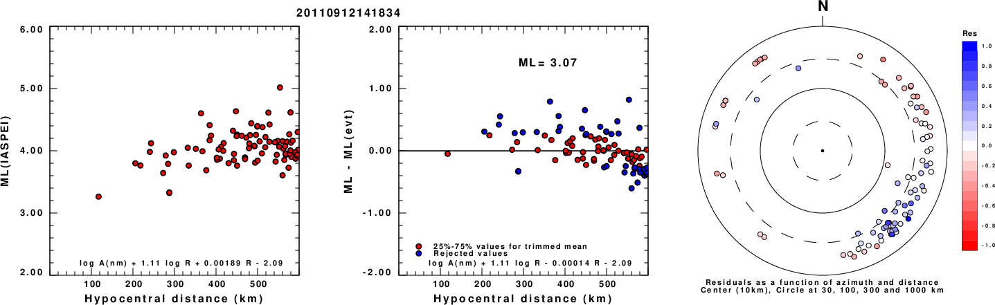
Left: ML computed using the IASPEI formula for Vertical components (research). Center: ML residuals computed using a modified IASPEI formula that accounts for path specific attenuation; the values used for the trimmed mean are indicated. The ML relation used for each figure is given at the bottom of each plot.
Right: Residuals from new relation as a function of distance and azimuth.
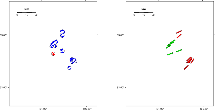 |
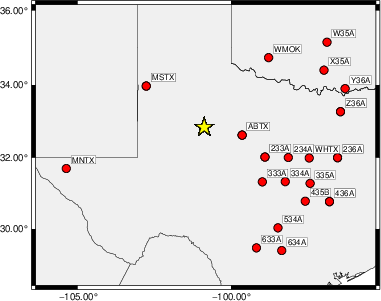
The focal mechanism was determined using broadband seismic waveforms. The location of the event (star) and the stations used for (red) the waveform inversion are shown in the next figure.
|
|
|
The program wvfgrd96 was used with good traces observed at short distance to determine the focal mechanism, depth and seismic moment. This technique requires a high quality signal and well determined velocity model for the Green's functions. To the extent that these are the quality data, this type of mechanism should be preferred over the radiation pattern technique which requires the separate step of defining the pressure and tension quadrants and the correct strike.
The observed and predicted traces are filtered using the following gsac commands:
cut o DIST/3.3 -40 o DIST/3.3 +50
rtr
taper w 0.1
hp c 0.03 n 3
lp c 0.10 n 3
br c 0.12 0.25 n 4 p 2
The results of this grid search are as follow:
           DEPTH  STK   DIP  RAKE   MW    FIT
WVFGRD96    0.5   115    80   -15   3.42 0.5932
WVFGRD96    1.0   115    80   -10   3.43 0.6071
WVFGRD96    2.0   295    90    15   3.45 0.6227
WVFGRD96    3.0   295    70    10   3.47 0.6331
WVFGRD96    4.0   115    70     0   3.48 0.6440
WVFGRD96    5.0   110    70   -15   3.49 0.6514
WVFGRD96    6.0   110    70   -10   3.50 0.6583
WVFGRD96    7.0   110    70   -10   3.51 0.6634
WVFGRD96    8.0   110    75   -25   3.53 0.6677
WVFGRD96    9.0   300    70    30   3.55 0.6696
WVFGRD96   10.0   300    70    30   3.57 0.6714
WVFGRD96   11.0   300    70    30   3.57 0.6706
WVFGRD96   12.0   300    75    25   3.57 0.6688
WVFGRD96   13.0   300    75    25   3.58 0.6659
WVFGRD96   14.0   300    75    25   3.59 0.6622
WVFGRD96   15.0   300    75    25   3.60 0.6572
WVFGRD96   16.0   300    75    25   3.60 0.6509
WVFGRD96   17.0   300    80    25   3.61 0.6434
WVFGRD96   18.0   300    80    25   3.62 0.6357
WVFGRD96   19.0   300    80    25   3.63 0.6265
WVFGRD96   20.0   305    75    25   3.65 0.6154
WVFGRD96   21.0   305    80    25   3.66 0.6045
WVFGRD96   22.0   305    80    30   3.68 0.5934
WVFGRD96   23.0   120    85   -40   3.71 0.5815
WVFGRD96   24.0   120    85   -40   3.71 0.5702
WVFGRD96   25.0   120    85   -45   3.73 0.5583
WVFGRD96   26.0   300    90    45   3.73 0.5447
WVFGRD96   27.0   300    90    50   3.75 0.5334
WVFGRD96   28.0   120    85   -50   3.76 0.5227
WVFGRD96   29.0   120    85   -50   3.77 0.5095
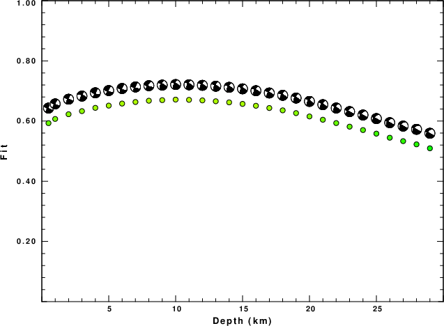
The best solution is
WVFGRD96 10.0 300 70 30 3.57 0.6714
The mechanism corresponding to the best fit is
|
|
|
The best fit as a function of depth is given in the following figure:
|
|
|
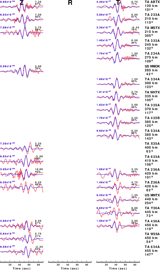
The comparison of the observed and predicted waveforms is given in the next figure. The red traces are the observed and the blue are the predicted. Each observed-predicted component is plotted to the same scale and peak amplitudes are indicated by the numbers to the left of each trace. A pair of numbers is given in black at the right of each predicted traces. The upper number it the time shift required for maximum correlation between the observed and predicted traces. This time shift is required because the synthetics are not computed at exactly the same distance as the observed, the velocity model used in the predictions may not be perfect and the epicentral parameters may be be off. A positive time shift indicates that the prediction is too fast and should be delayed to match the observed trace (shift to the right in this figure). A negative value indicates that the prediction is too slow. The lower number gives the percentage of variance reduction to characterize the individual goodness of fit (100% indicates a perfect fit).
The bandpass filter used in the processing and for the display was
cut o DIST/3.3 -40 o DIST/3.3 +50
rtr
taper w 0.1
hp c 0.03 n 3
lp c 0.10 n 3
br c 0.12 0.25 n 4 p 2
|
| Figure 3. Waveform comparison for selected depth. Red: observed; Blue - predicted. The time shift with respect to the model prediction is indicated. The percent of fit is also indicated. The time scale is relative to the first trace sample. |
|
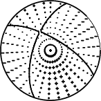
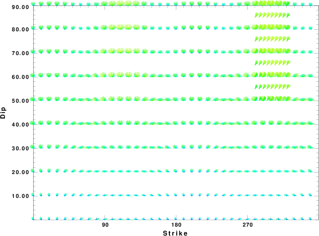
| Focal mechanism sensitivity at the preferred depth. The red color indicates a very good fit to the waveforms. Each solution is plotted as a vector at a given value of strike and dip with the angle of the vector representing the rake angle, measured, with respect to the upward vertical (N) in the figure. |
The CUS model used for the waveform synthetic seismograms and for the surface wave eigenfunctions and dispersion is as follows (The format is in the model96 format of Computer Programs in Seismology).
MODEL.01
CUS Model with Q from simple gamma values
ISOTROPIC
KGS
FLAT EARTH
1-D
CONSTANT VELOCITY
LINE08
LINE09
LINE10
LINE11
  H(KM) VP(KM/S) VS(KM/S) RHO(GM/CC)   QP   QS  ETAP  ETAS  FREFP  FREFS
  1.0000  5.0000  2.8900  2.5000 0.172E-02 0.387E-02 0.00  0.00  1.00  1.00
  9.0000  6.1000  3.5200  2.7300 0.160E-02 0.363E-02 0.00  0.00  1.00  1.00
 10.0000  6.4000  3.7000  2.8200 0.149E-02 0.336E-02 0.00  0.00  1.00  1.00
 20.0000  6.7000  3.8700  2.9020 0.000E-04 0.000E-04 0.00  0.00  1.00  1.00
  0.0000  8.1500  4.7000  3.3640 0.194E-02 0.431E-02 0.00  0.00  1.00  1.00