Location
Location ANSS
The ANSS event ID is ak0119lvnlpb and the event page is at
https://earthquake.usgs.gov/earthquakes/eventpage/ak0119lvnlpb/executive.
2011/07/28 14:00:00 62.048 -151.303 86.5 5.3 Alaska
Focal Mechanism
 USGS/SLU Moment Tensor Solution
 ENS  2011/07/28 14:00:00:0  62.05 -151.30  86.5 5.3 Alaska

 Stations used:
   AK.BAL AK.BMR AK.BRLK AK.CAST AK.CCB AK.CHUM AK.CNP AK.COLD
   AK.CRQ AK.CTG AK.DHY AK.DIV AK.EYAK AK.FIB AK.FID AK.FYU
   AK.GHO AK.HOM AK.KLU AK.KNK AK.KTH AK.MCK AK.MDM AK.MLY
   AK.PAX AK.PPLA AK.RAG AK.RC01 AK.RND AK.SAW AK.SCM AK.SSN
   AK.SWD AK.TGL AK.TRF AK.WRH AT.MENT AT.OHAK AT.PMR AT.SVW2
   IU.COLA US.EGAK

 Filtering commands used:
   cut o DIST/3.3 -40 o DIST/3.3 +50
   rtr
   taper w 0.1
   hp c 0.03 n 3
   lp c 0.06 n 3

 Best Fitting Double Couple
  Mo = 8.81e+23 dyne-cm
  Mw = 5.23
  Z  = 84 km
  Plane   Strike  Dip  Rake
   NP1      348    70   105
   NP2      130    25    55
  Principal Axes:
   Axis    Value   Plunge  Azimuth
    T   8.81e+23     62     281
    N   0.00e+00     14     162
    P  -8.81e+23     23      66

 Moment Tensor: (dyne-cm)
    Component   Value
       Mxx    -1.14e+23
       Mxy    -3.09e+23
       Mxz    -6.10e+22
       Myy    -4.39e+23
       Myz    -6.49e+23
       Mzz     5.53e+23


                     ###-----------
                 #########-------------
              #############---------------
             ###############---------------
           ##################----------------
          -###################----------------
         -#####################----------   ---
        --######################--------- P ----
        --######################---------   ----
       ---##########   ##########----------------
       ---########## T ##########----------------
       ----#########   ##########----------------
       ----#######################---------------
        ----######################--------------
        -----#####################--------------
         -----####################-------------
          ------##################------------
           -------################-----------
             -------##############---------
              ----------##########------##
                 ----------------######
                     ------------##


 Global CMT Convention Moment Tensor:
      R          T          P
  5.53e+23  -6.10e+22   6.49e+23
 -6.10e+22  -1.14e+23   3.09e+23
  6.49e+23   3.09e+23  -4.39e+23


Details of the solution is found at

http://www.eas.slu.edu/eqc/eqc_mt/MECH.NA/20110728140000/index.html
|
Preferred Solution
The preferred solution from an analysis of the surface-wave spectral amplitude radiation pattern, waveform inversion or first motion observations is
      STK = 130
      DIP = 25
     RAKE = 55
       MW = 5.23
       HS = 84.0
The NDK file is 20110728140000.ndk
The waveform inversion is preferred.
Magnitudes
Given the availability of digital waveforms for determination of the moment tensor, this section documents the added processing leading to mLg, if appropriate to the region, and ML by application of the respective IASPEI formulae. As a research study, the linear distance term of the IASPEI formula
for ML is adjusted to remove a linear distance trend in residuals to give a regionally defined ML. The defined ML uses horizontal component recordings, but the same procedure is applied to the vertical components since there may be some interest in vertical component ground motions. Residual plots versus distance may indicate interesting features of ground motion scaling in some distance ranges. A residual plot of the regionalized magnitude is given as a function of distance and azimuth, since data sets may transcend different wave propagation provinces.
ML Magnitude
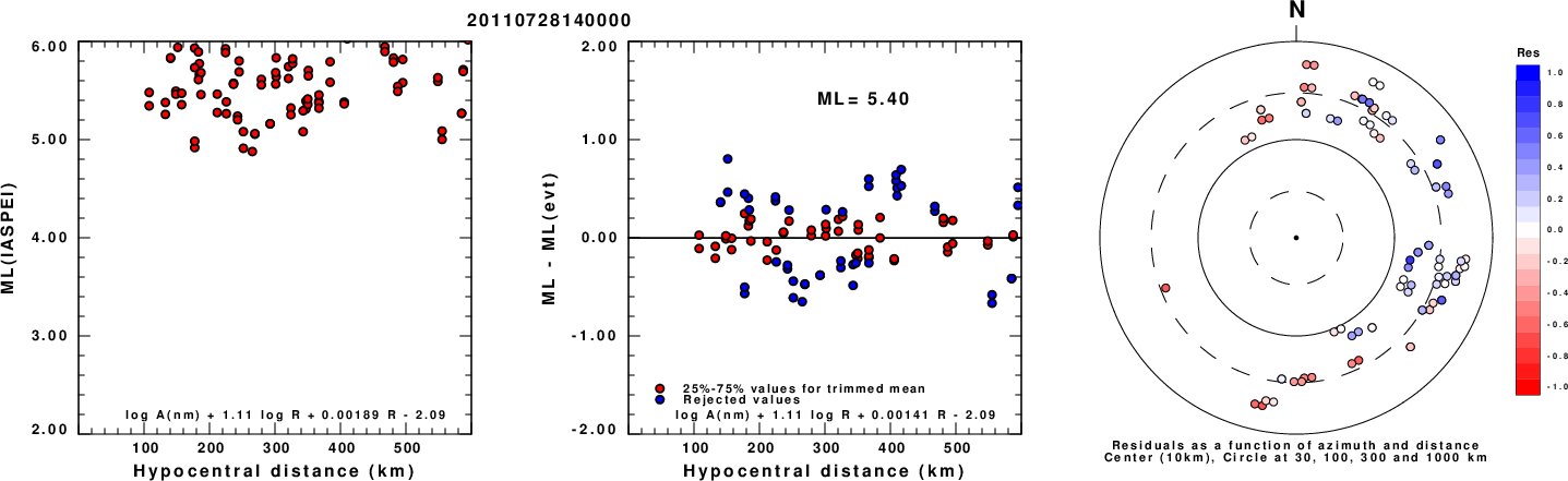
Left: ML computed using the IASPEI formula for Horizontal components. Center: ML residuals computed using a modified IASPEI formula that accounts for path specific attenuation; the values used for the trimmed mean are indicated. The ML relation used for each figure is given at the bottom of each plot.
Right: Residuals from new relation as a function of distance and azimuth.
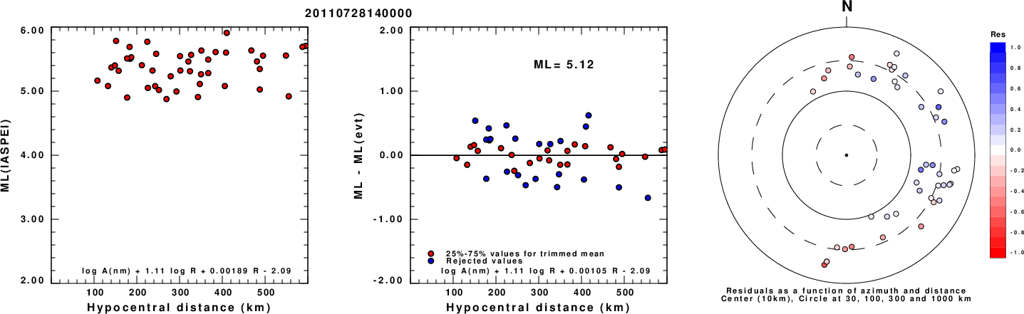
Left: ML computed using the IASPEI formula for Vertical components (research). Center: ML residuals computed using a modified IASPEI formula that accounts for path specific attenuation; the values used for the trimmed mean are indicated. The ML relation used for each figure is given at the bottom of each plot.
Right: Residuals from new relation as a function of distance and azimuth.
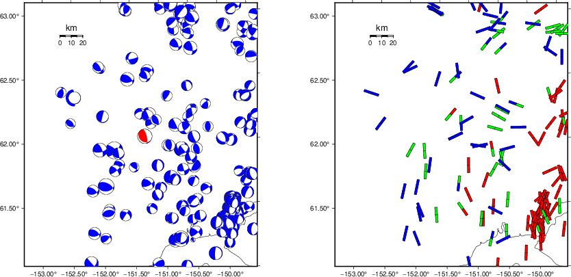
Context
The left panel of the next figure presents the focal mechanism for this earthquake (red) in the context of other nearby events (blue) in the SLU Moment Tensor Catalog. The right panel shows the inferred direction of maximum compressive stress and the type of faulting (green is strike-slip, red is normal, blue is thrust; oblique is shown by a combination of colors). Thus context plot is useful for assessing the appropriateness of the moment tensor of this event.
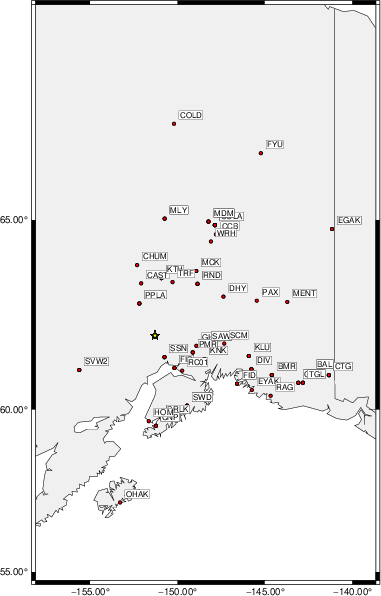
Waveform Inversion using wvfgrd96
The focal mechanism was determined using broadband seismic waveforms. The location of the event (star) and the
stations used for (red) the waveform inversion are shown in the next figure.
|
|
Location of broadband stations used for waveform inversion
|
The program wvfgrd96 was used with good traces observed at short distance to determine the focal mechanism, depth and seismic moment. This technique requires a high quality signal and well determined velocity model for the Green's functions. To the extent that these are the quality data, this type of mechanism should be preferred over the radiation pattern technique which requires the separate step of defining the pressure and tension quadrants and the correct strike.
The observed and predicted traces are filtered using the following gsac commands:
cut o DIST/3.3 -40 o DIST/3.3 +50
rtr
taper w 0.1
hp c 0.03 n 3
lp c 0.06 n 3
The results of this grid search are as follow:
           DEPTH  STK   DIP  RAKE   MW    FIT
WVFGRD96    1.0    40    45   -70   4.34 0.2072
WVFGRD96    3.0    40    50   -60   4.50 0.2543
WVFGRD96    4.0   235    70   -45   4.49 0.2417
WVFGRD96    7.0    70    80    30   4.53 0.2689
WVFGRD96    9.0    70    75    35   4.58 0.2782
WVFGRD96   11.0    70    75    35   4.60 0.2832
WVFGRD96   13.0    75    70    35   4.61 0.2824
WVFGRD96   15.0    75    70    35   4.63 0.2798
WVFGRD96   17.0    80    70    30   4.64 0.2770
WVFGRD96   19.0   250    60    40   4.66 0.2759
WVFGRD96   21.0   250    65    35   4.68 0.2769
WVFGRD96   23.0   250    65    40   4.69 0.2777
WVFGRD96   25.0   250    65    35   4.71 0.2781
WVFGRD96   27.0   250    65    40   4.72 0.2777
WVFGRD96   29.0   250    65    40   4.74 0.2769
WVFGRD96   31.0    80    85    25   4.76 0.2787
WVFGRD96   33.0    80    80    20   4.78 0.2828
WVFGRD96   35.0    80    85    20   4.81 0.2901
WVFGRD96   37.0    80    85    20   4.83 0.2970
WVFGRD96   39.0    80    80    15   4.87 0.3051
WVFGRD96   41.0    75    40   -20   4.94 0.3044
WVFGRD96   43.0    80    45   -10   4.96 0.3084
WVFGRD96   45.0    85    40     0   4.98 0.3197
WVFGRD96   47.0    85    40     0   5.00 0.3327
WVFGRD96   49.0    90    40     5   5.02 0.3456
WVFGRD96   51.0    90    40    10   5.04 0.3597
WVFGRD96   53.0    90    35    10   5.06 0.3737
WVFGRD96   55.0    90    35    10   5.07 0.3875
WVFGRD96   57.0    95    35    20   5.09 0.4005
WVFGRD96   59.0   100    35    30   5.11 0.4147
WVFGRD96   61.0   100    35    30   5.12 0.4332
WVFGRD96   63.0   120    20    40   5.15 0.4511
WVFGRD96   65.0   125    20    50   5.17 0.4728
WVFGRD96   67.0   125    20    50   5.18 0.4924
WVFGRD96   69.0   125    20    50   5.19 0.5088
WVFGRD96   70.0   130    20    55   5.19 0.5161
WVFGRD96   71.0   130    20    55   5.20 0.5230
WVFGRD96   72.0   130    20    55   5.20 0.5288
WVFGRD96   73.0   130    20    55   5.20 0.5348
WVFGRD96   74.0   130    20    55   5.21 0.5391
WVFGRD96   75.0   130    20    55   5.21 0.5436
WVFGRD96   76.0   130    20    55   5.21 0.5469
WVFGRD96   77.0   125    25    50   5.21 0.5504
WVFGRD96   78.0   125    25    50   5.21 0.5534
WVFGRD96   79.0   125    25    50   5.22 0.5560
WVFGRD96   80.0   125    25    50   5.22 0.5578
WVFGRD96   81.0   130    25    55   5.22 0.5597
WVFGRD96   82.0   130    25    55   5.22 0.5609
WVFGRD96   83.0   130    25    55   5.22 0.5613
WVFGRD96   84.0   130    25    55   5.23 0.5619
WVFGRD96   85.0   130    25    55   5.23 0.5618
WVFGRD96   86.0   130    25    55   5.23 0.5616
WVFGRD96   87.0   130    25    55   5.23 0.5609
WVFGRD96   88.0   130    25    55   5.23 0.5598
WVFGRD96   89.0   130    25    55   5.23 0.5587
WVFGRD96   90.0   130    25    55   5.23 0.5566
WVFGRD96   91.0   130    25    55   5.23 0.5550
WVFGRD96   92.0   130    25    55   5.23 0.5530
WVFGRD96   93.0   130    25    55   5.23 0.5502
WVFGRD96   94.0   130    25    55   5.23 0.5482
WVFGRD96   95.0   130    25    55   5.23 0.5451
WVFGRD96   96.0   130    25    55   5.23 0.5423
WVFGRD96   97.0   130    25    55   5.23 0.5395
WVFGRD96   98.0   130    25    55   5.23 0.5360
WVFGRD96   99.0   130    25    55   5.23 0.5327
WVFGRD96  100.0   130    25    55   5.23 0.5296
WVFGRD96  101.0   130    25    55   5.23 0.5256
WVFGRD96  102.0   130    25    55   5.23 0.5226
WVFGRD96  103.0   135    25    60   5.23 0.5187
WVFGRD96  104.0   135    25    60   5.23 0.5152
WVFGRD96  105.0   135    25    60   5.23 0.5114
WVFGRD96  106.0   135    25    60   5.23 0.5085
WVFGRD96  107.0   135    25    60   5.23 0.5042
WVFGRD96  108.0   135    25    60   5.23 0.5017
WVFGRD96  109.0   135    25    60   5.23 0.4977
WVFGRD96  111.0   135    25    60   5.23 0.4906
WVFGRD96  113.0   135    25    60   5.23 0.4836
WVFGRD96  115.0   135    25    60   5.23 0.4769
WVFGRD96  117.0   125    30    55   5.23 0.4696
WVFGRD96  119.0   125    30    55   5.23 0.4631
WVFGRD96  121.0   135    25    65   5.23 0.4564
WVFGRD96  123.0   135    25    65   5.23 0.4497
WVFGRD96  125.0   135    25    65   5.22 0.4429
WVFGRD96  127.0   140    25    70   5.22 0.4361
WVFGRD96  129.0   140    25    70   5.22 0.4297
The best solution is
WVFGRD96 84.0 130 25 55 5.23 0.5619
The mechanism corresponding to the best fit is
|
|
Figure 1. Waveform inversion focal mechanism
|
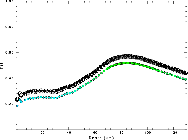
The best fit as a function of depth is given in the following figure:
|
|
Figure 2. Depth sensitivity for waveform mechanism
|
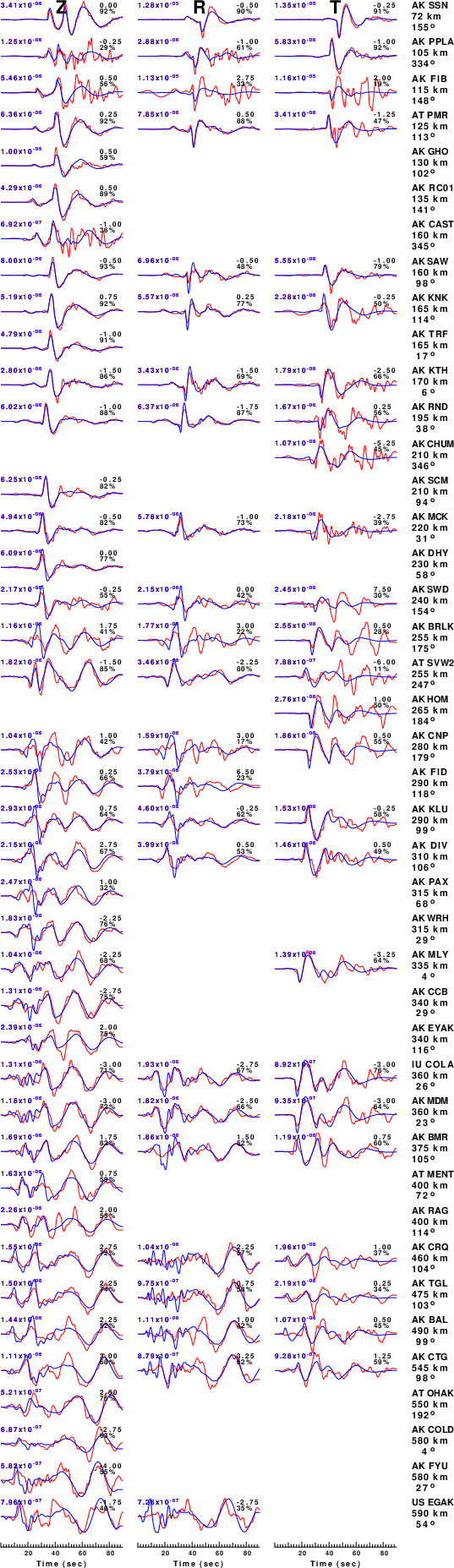
The comparison of the observed and predicted waveforms is given in the next figure. The red traces are the observed and the blue are the predicted.
Each observed-predicted component is plotted to the same scale and peak amplitudes are indicated by the numbers to the left of each trace. A pair of numbers is given in black at the right of each predicted traces. The upper number it the time shift required for maximum correlation between the observed and predicted traces. This time shift is required because the synthetics are not computed at exactly the same distance as the observed, the velocity model used in the predictions may not be perfect and the epicentral parameters may be be off.
A positive time shift indicates that the prediction is too fast and should be delayed to match the observed trace (shift to the right in this figure). A negative value indicates that the prediction is too slow. The lower number gives the percentage of variance reduction to characterize the individual goodness of fit (100% indicates a perfect fit).
The bandpass filter used in the processing and for the display was
cut o DIST/3.3 -40 o DIST/3.3 +50
rtr
taper w 0.1
hp c 0.03 n 3
lp c 0.06 n 3
|
|
Figure 3. Waveform comparison for selected depth. Red: observed; Blue - predicted. The time shift with respect to the model prediction is indicated. The percent of fit is also indicated. The time scale is relative to the first trace sample.
|
|
|
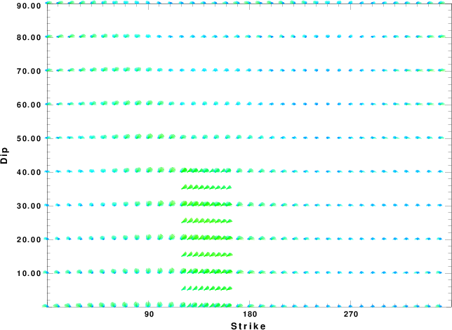
Focal mechanism sensitivity at the preferred depth. The red color indicates a very good fit to the waveforms.
Each solution is plotted as a vector at a given value of strike and dip with the angle of the vector representing the rake angle, measured, with respect to the upward vertical (N) in the figure.
|
A check on the assumed source location is possible by looking at the time shifts between the observed and predicted traces. The time shifts for waveform matching arise for several reasons:
- The origin time and epicentral distance are incorrect
- The velocity model used for the inversion is incorrect
- The velocity model used to define the P-arrival time is not the
same as the velocity model used for the waveform inversion
(assuming that the initial trace alignment is based on the
P arrival time)
Assuming only a mislocation, the time shifts are fit to a functional form:
Time_shift = A + B cos Azimuth + C Sin Azimuth
The time shifts for this inversion lead to the next figure:
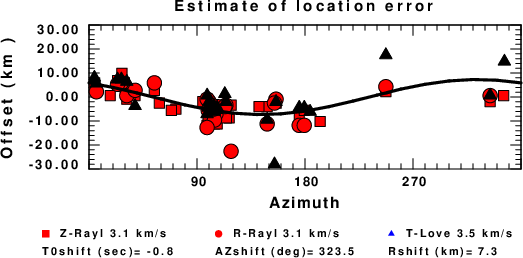
The derived shift in origin time and epicentral coordinates are given at the bottom of the figure.
Velocity Model
The WUS.model used for the waveform synthetic seismograms and for the surface wave eigenfunctions and dispersion is as follows
(The format is in the model96 format of Computer Programs in Seismology).
MODEL.01
Model after     8 iterations
ISOTROPIC
KGS
FLAT EARTH
1-D
CONSTANT VELOCITY
LINE08
LINE09
LINE10
LINE11
      H(KM)   VP(KM/S)   VS(KM/S) RHO(GM/CC)         QP         QS       ETAP       ETAS      FREFP      FREFS
     1.9000     3.4065     2.0089     2.2150  0.302E-02  0.679E-02   0.00       0.00       1.00       1.00
     6.1000     5.5445     3.2953     2.6089  0.349E-02  0.784E-02   0.00       0.00       1.00       1.00
    13.0000     6.2708     3.7396     2.7812  0.212E-02  0.476E-02   0.00       0.00       1.00       1.00
    19.0000     6.4075     3.7680     2.8223  0.111E-02  0.249E-02   0.00       0.00       1.00       1.00
     0.0000     7.9000     4.6200     3.2760  0.164E-10  0.370E-10   0.00       0.00       1.00       1.00
Last Changed Sat Apr 27 03:06:04 PM CDT 2024