Location
Location ANSS
The ANSS event ID is ak0119a690lk and the event page is at
https://earthquake.usgs.gov/earthquakes/eventpage/ak0119a690lk/executive.
2011/07/21 06:20:11 60.031 -152.831 92.7 3.7 Alaska
Focal Mechanism
 USGS/SLU Moment Tensor Solution
 ENS  2011/07/21 06:20:11:0  60.03 -152.83  92.7 3.7 Alaska

 Stations used:
   AK.CNP AK.FIB AK.GHO AK.HOM AK.SAW AK.SKN AK.SSN AK.SWD
   AT.PMR AT.SVW2 II.KDAK

 Filtering commands used:
   hp c 0.02 n 3
   lp c 0.10 n 3

 Best Fitting Double Couple
  Mo = 3.31e+22 dyne-cm
  Mw = 4.28
  Z  = 116 km
  Plane   Strike  Dip  Rake
   NP1       55    60    40
   NP2      302    56   143
  Principal Axes:
   Axis    Value   Plunge  Azimuth
    T   3.31e+22     48     270
    N   0.00e+00     42      86
    P  -3.31e+22      2     178

 Moment Tensor: (dyne-cm)
    Component   Value
       Mxx    -3.30e+22
       Mxy     1.15e+21
       Mxz     1.44e+21
       Myy     1.46e+22
       Myz    -1.65e+22
       Mzz     1.84e+22


                     --------------
                 ----------------------
              ----------------------------
             ------------------------------
           ---######-------------------------
          #################------------------#
         ######################-------------###
        ##########################---------#####
        ############################-------#####
       #########   ###################---########
       ######### T ##############################
       #########   ###################---########
       ##############################------######
        ##########################----------####
        ########################-------------###
         ####################----------------##
          ###############--------------------#
           ########--------------------------
             ------------------------------
              ----------------------------
                 ----------   ---------
                     ------ P -----


 Global CMT Convention Moment Tensor:
      R          T          P
  1.84e+22   1.44e+21   1.65e+22
  1.44e+21  -3.30e+22  -1.15e+21
  1.65e+22  -1.15e+21   1.46e+22


Details of the solution is found at

http://www.eas.slu.edu/eqc/eqc_mt/MECH.NA/20110721062011/index.html
|
Preferred Solution
The preferred solution from an analysis of the surface-wave spectral amplitude radiation pattern, waveform inversion or first motion observations is
      STK = 55
      DIP = 60
     RAKE = 40
       MW = 4.28
       HS = 116.0
The NDK file is 20110721062011.ndk
The waveform inversion is preferred.
Magnitudes
Given the availability of digital waveforms for determination of the moment tensor, this section documents the added processing leading to mLg, if appropriate to the region, and ML by application of the respective IASPEI formulae. As a research study, the linear distance term of the IASPEI formula
for ML is adjusted to remove a linear distance trend in residuals to give a regionally defined ML. The defined ML uses horizontal component recordings, but the same procedure is applied to the vertical components since there may be some interest in vertical component ground motions. Residual plots versus distance may indicate interesting features of ground motion scaling in some distance ranges. A residual plot of the regionalized magnitude is given as a function of distance and azimuth, since data sets may transcend different wave propagation provinces.
ML Magnitude
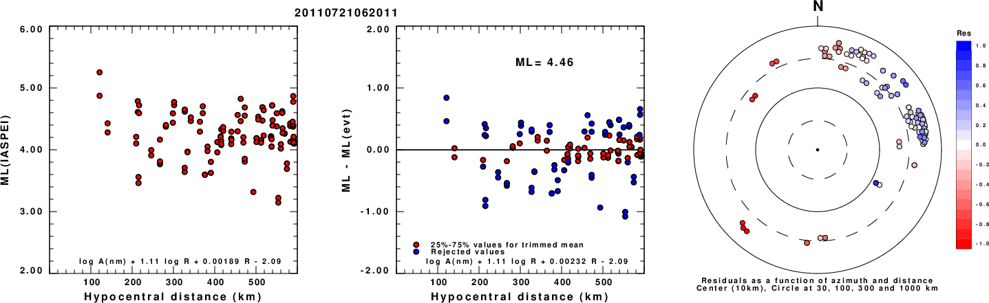
Left: ML computed using the IASPEI formula for Horizontal components. Center: ML residuals computed using a modified IASPEI formula that accounts for path specific attenuation; the values used for the trimmed mean are indicated. The ML relation used for each figure is given at the bottom of each plot.
Right: Residuals from new relation as a function of distance and azimuth.
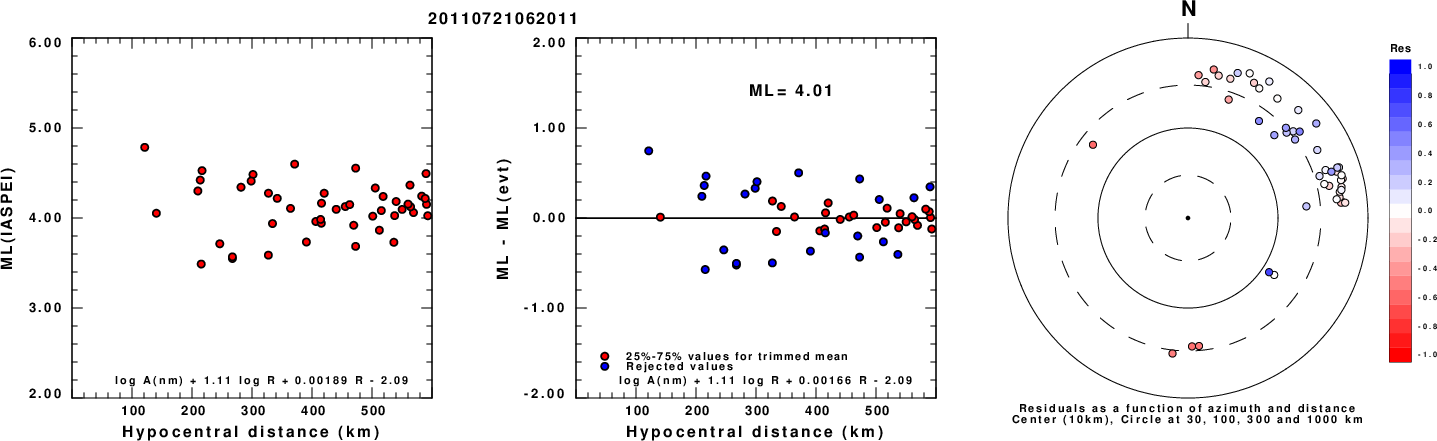
Left: ML computed using the IASPEI formula for Vertical components (research). Center: ML residuals computed using a modified IASPEI formula that accounts for path specific attenuation; the values used for the trimmed mean are indicated. The ML relation used for each figure is given at the bottom of each plot.
Right: Residuals from new relation as a function of distance and azimuth.
Context
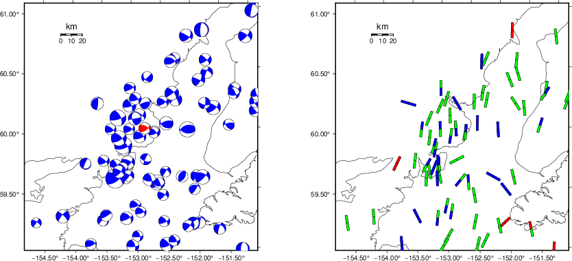
The left panel of the next figure presents the focal mechanism for this earthquake (red) in the context of other nearby events (blue) in the SLU Moment Tensor Catalog. The right panel shows the inferred direction of maximum compressive stress and the type of faulting (green is strike-slip, red is normal, blue is thrust; oblique is shown by a combination of colors). Thus context plot is useful for assessing the appropriateness of the moment tensor of this event.
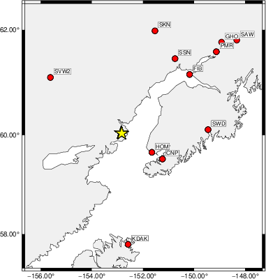
Waveform Inversion using wvfgrd96
The focal mechanism was determined using broadband seismic waveforms. The location of the event (star) and the
stations used for (red) the waveform inversion are shown in the next figure.
|
|
Location of broadband stations used for waveform inversion
|
The program wvfgrd96 was used with good traces observed at short distance to determine the focal mechanism, depth and seismic moment. This technique requires a high quality signal and well determined velocity model for the Green's functions. To the extent that these are the quality data, this type of mechanism should be preferred over the radiation pattern technique which requires the separate step of defining the pressure and tension quadrants and the correct strike.
The observed and predicted traces are filtered using the following gsac commands:
hp c 0.02 n 3
lp c 0.10 n 3
The results of this grid search are as follow:
           DEPTH  STK   DIP  RAKE   MW    FIT
WVFGRD96   50.0    50    70   -10   4.10 0.2975
WVFGRD96   51.0    50    70   -10   4.11 0.2985
WVFGRD96   52.0   225    70   -10   4.15 0.3004
WVFGRD96   53.0   225    70   -10   4.15 0.3013
WVFGRD96   54.0   220    70   -20   4.15 0.3042
WVFGRD96   55.0   220    70   -20   4.16 0.3067
WVFGRD96   56.0   220    70   -20   4.17 0.3084
WVFGRD96   57.0   220    75   -25   4.17 0.3123
WVFGRD96   58.0   220    75   -25   4.17 0.3158
WVFGRD96   59.0   220    75   -25   4.18 0.3175
WVFGRD96   60.0   220    75   -25   4.18 0.3209
WVFGRD96   61.0   220    75   -25   4.19 0.3237
WVFGRD96   62.0   220    75   -25   4.20 0.3258
WVFGRD96   63.0   220    75   -25   4.20 0.3286
WVFGRD96   64.0   220    75   -25   4.20 0.3285
WVFGRD96   65.0   220    80   -25   4.19 0.3321
WVFGRD96   66.0   220    80   -25   4.20 0.3336
WVFGRD96   67.0   220    80   -25   4.20 0.3354
WVFGRD96   68.0   220    80   -25   4.21 0.3374
WVFGRD96   69.0   220    80   -25   4.21 0.3388
WVFGRD96   70.0   220    80   -25   4.21 0.3399
WVFGRD96   71.0    55    80    20   4.22 0.3440
WVFGRD96   72.0    55    75    20   4.21 0.3466
WVFGRD96   73.0    55    75    20   4.22 0.3473
WVFGRD96   74.0    55    75    20   4.22 0.3507
WVFGRD96   75.0    50    70    30   4.19 0.3525
WVFGRD96   76.0    50    70    30   4.19 0.3549
WVFGRD96   77.0    50    70    30   4.20 0.3572
WVFGRD96   78.0    50    70    30   4.20 0.3585
WVFGRD96   79.0    50    70    30   4.20 0.3614
WVFGRD96   80.0    50    70    30   4.20 0.3629
WVFGRD96   81.0    55    70    30   4.23 0.3653
WVFGRD96   82.0    50    70    35   4.21 0.3664
WVFGRD96   83.0    55    65    35   4.22 0.3687
WVFGRD96   84.0    55    65    35   4.22 0.3700
WVFGRD96   85.0    55    65    35   4.22 0.3724
WVFGRD96   86.0    55    65    35   4.23 0.3744
WVFGRD96   87.0    55    65    35   4.23 0.3755
WVFGRD96   88.0    55    65    35   4.23 0.3778
WVFGRD96   89.0    55    65    35   4.23 0.3783
WVFGRD96   90.0    55    65    35   4.24 0.3818
WVFGRD96   91.0    55    65    35   4.24 0.3822
WVFGRD96   92.0    55    65    35   4.24 0.3848
WVFGRD96   93.0    55    65    35   4.24 0.3866
WVFGRD96   94.0    55    65    35   4.25 0.3875
WVFGRD96   95.0    55    65    35   4.25 0.3894
WVFGRD96   96.0    55    65    35   4.25 0.3911
WVFGRD96   97.0    55    65    35   4.25 0.3919
WVFGRD96   98.0    55    60    35   4.24 0.3943
WVFGRD96   99.0    55    60    35   4.24 0.3936
WVFGRD96  100.0    55    60    35   4.24 0.3970
WVFGRD96  101.0    55    60    35   4.24 0.3978
WVFGRD96  102.0    55    60    40   4.25 0.3982
WVFGRD96  103.0    55    60    40   4.25 0.4004
WVFGRD96  104.0    55    60    40   4.25 0.4022
WVFGRD96  105.0    55    60    40   4.25 0.4019
WVFGRD96  106.0    55    60    40   4.26 0.4043
WVFGRD96  107.0    55    60    40   4.26 0.4054
WVFGRD96  108.0    55    60    40   4.26 0.4045
WVFGRD96  109.0    55    60    40   4.26 0.4074
WVFGRD96  110.0    55    60    40   4.27 0.4073
WVFGRD96  111.0    55    60    40   4.27 0.4073
WVFGRD96  112.0    55    60    40   4.27 0.4089
WVFGRD96  113.0    55    60    40   4.27 0.4093
WVFGRD96  114.0    55    60    40   4.27 0.4082
WVFGRD96  115.0    55    60    40   4.28 0.4096
WVFGRD96  116.0    55    60    40   4.28 0.4101
WVFGRD96  117.0    55    60    40   4.28 0.4090
WVFGRD96  118.0    55    60    40   4.28 0.4100
WVFGRD96  119.0    55    60    40   4.28 0.4100
WVFGRD96  120.0    55    60    40   4.28 0.4088
WVFGRD96  121.0    55    60    40   4.29 0.4091
WVFGRD96  122.0    55    60    40   4.29 0.4094
WVFGRD96  123.0    50    60    40   4.28 0.4086
WVFGRD96  124.0    50    60    40   4.28 0.4082
WVFGRD96  125.0    50    60    40   4.28 0.4088
WVFGRD96  126.0    50    60    40   4.28 0.4083
WVFGRD96  127.0    50    60    40   4.28 0.4075
WVFGRD96  128.0    50    60    40   4.28 0.4068
WVFGRD96  129.0    55    55    40   4.28 0.4073
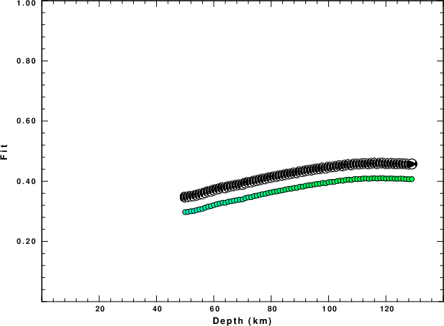
The best solution is
WVFGRD96 116.0 55 60 40 4.28 0.4101
The mechanism corresponding to the best fit is
|
|
Figure 1. Waveform inversion focal mechanism
|
The best fit as a function of depth is given in the following figure:
|
|
Figure 2. Depth sensitivity for waveform mechanism
|
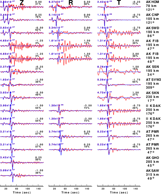
The comparison of the observed and predicted waveforms is given in the next figure. The red traces are the observed and the blue are the predicted.
Each observed-predicted component is plotted to the same scale and peak amplitudes are indicated by the numbers to the left of each trace. A pair of numbers is given in black at the right of each predicted traces. The upper number it the time shift required for maximum correlation between the observed and predicted traces. This time shift is required because the synthetics are not computed at exactly the same distance as the observed, the velocity model used in the predictions may not be perfect and the epicentral parameters may be be off.
A positive time shift indicates that the prediction is too fast and should be delayed to match the observed trace (shift to the right in this figure). A negative value indicates that the prediction is too slow. The lower number gives the percentage of variance reduction to characterize the individual goodness of fit (100% indicates a perfect fit).
The bandpass filter used in the processing and for the display was
hp c 0.02 n 3
lp c 0.10 n 3
|
|
Figure 3. Waveform comparison for selected depth. Red: observed; Blue - predicted. The time shift with respect to the model prediction is indicated. The percent of fit is also indicated. The time scale is relative to the first trace sample.
|
|
|
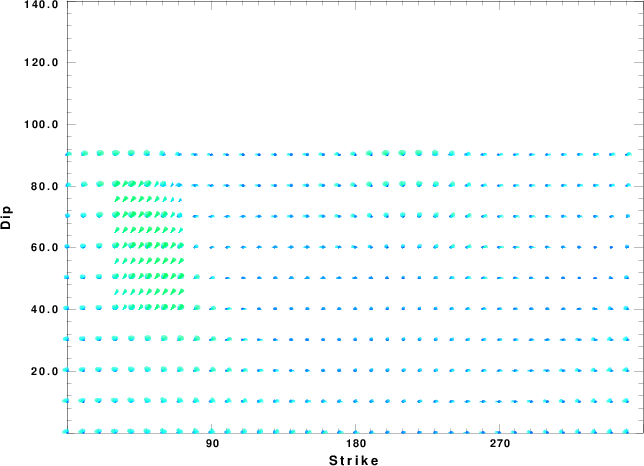
Focal mechanism sensitivity at the preferred depth. The red color indicates a very good fit to the waveforms.
Each solution is plotted as a vector at a given value of strike and dip with the angle of the vector representing the rake angle, measured, with respect to the upward vertical (N) in the figure.
|
A check on the assumed source location is possible by looking at the time shifts between the observed and predicted traces. The time shifts for waveform matching arise for several reasons:
- The origin time and epicentral distance are incorrect
- The velocity model used for the inversion is incorrect
- The velocity model used to define the P-arrival time is not the
same as the velocity model used for the waveform inversion
(assuming that the initial trace alignment is based on the
P arrival time)
Assuming only a mislocation, the time shifts are fit to a functional form:
Time_shift = A + B cos Azimuth + C Sin Azimuth
The time shifts for this inversion lead to the next figure:
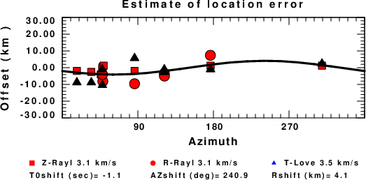
The derived shift in origin time and epicentral coordinates are given at the bottom of the figure.
Velocity Model
The WUS.model used for the waveform synthetic seismograms and for the surface wave eigenfunctions and dispersion is as follows
(The format is in the model96 format of Computer Programs in Seismology).
MODEL.01
Model after     8 iterations
ISOTROPIC
KGS
FLAT EARTH
1-D
CONSTANT VELOCITY
LINE08
LINE09
LINE10
LINE11
      H(KM)   VP(KM/S)   VS(KM/S) RHO(GM/CC)         QP         QS       ETAP       ETAS      FREFP      FREFS
     1.9000     3.4065     2.0089     2.2150  0.302E-02  0.679E-02   0.00       0.00       1.00       1.00
     6.1000     5.5445     3.2953     2.6089  0.349E-02  0.784E-02   0.00       0.00       1.00       1.00
    13.0000     6.2708     3.7396     2.7812  0.212E-02  0.476E-02   0.00       0.00       1.00       1.00
    19.0000     6.4075     3.7680     2.8223  0.111E-02  0.249E-02   0.00       0.00       1.00       1.00
     0.0000     7.9000     4.6200     3.2760  0.164E-10  0.370E-10   0.00       0.00       1.00       1.00
Last Changed Sat Apr 27 02:42:50 PM CDT 2024