Location
Location ANSS
The ANSS event ID is ak0118i0juhl and the event page is at
https://earthquake.usgs.gov/earthquakes/eventpage/ak0118i0juhl/executive.
2011/07/04 03:57:55 60.238 -152.802 111.9 4.2 Alaska
Focal Mechanism
 USGS/SLU Moment Tensor Solution
 ENS  2011/07/04 03:57:55:0  60.24 -152.80 111.9 4.2 Alaska

 Stations used:
   AK.BPAW AK.CAST AK.CNP AK.KTH AK.PPLA AK.RC01 AK.SSN AK.TRF
   AT.OHAK AT.PMR AT.SVW2 II.KDAK

 Filtering commands used:
   hp c 0.02 n 3
   lp c 0.06 n 3

 Best Fitting Double Couple
  Mo = 2.43e+22 dyne-cm
  Mw = 4.19
  Z  = 124 km
  Plane   Strike  Dip  Rake
   NP1      259    71   114
   NP2       25    30    40
  Principal Axes:
   Axis    Value   Plunge  Azimuth
    T   2.43e+22     57     201
    N   0.00e+00     23      71
    P  -2.43e+22     23     331

 Moment Tensor: (dyne-cm)
    Component   Value
       Mxx    -9.53e+21
       Mxy     1.11e+22
       Mxz    -1.79e+22
       Myy    -3.98e+21
       Myz     2.65e+20
       Mzz     1.35e+22


                     --------------
                 ---------------------#
              ----   -------------------##
             ----- P --------------------##
           -------   ---------------------###
          --------------------------------####
         ----------------------------------####
        -----------------------------------#####
        -------------------################----#
       -------------#######################------
       --------############################------
       -----###############################------
       --##################################------
        ##################################------
        ###############   ###############-------
         ############## T ##############-------
          #############   #############-------
           ##########################--------
             #######################-------
              ###################---------
                 #############---------
                     --------------


 Global CMT Convention Moment Tensor:
      R          T          P
  1.35e+22  -1.79e+22  -2.65e+20
 -1.79e+22  -9.53e+21  -1.11e+22
 -2.65e+20  -1.11e+22  -3.98e+21


Details of the solution is found at

http://www.eas.slu.edu/eqc/eqc_mt/MECH.NA/20110704035755/index.html
|
Preferred Solution
The preferred solution from an analysis of the surface-wave spectral amplitude radiation pattern, waveform inversion or first motion observations is
      STK = 25
      DIP = 30
     RAKE = 40
       MW = 4.19
       HS = 124.0
The NDK file is 20110704035755.ndk
The waveform inversion is preferred.
Magnitudes
Given the availability of digital waveforms for determination of the moment tensor, this section documents the added processing leading to mLg, if appropriate to the region, and ML by application of the respective IASPEI formulae. As a research study, the linear distance term of the IASPEI formula
for ML is adjusted to remove a linear distance trend in residuals to give a regionally defined ML. The defined ML uses horizontal component recordings, but the same procedure is applied to the vertical components since there may be some interest in vertical component ground motions. Residual plots versus distance may indicate interesting features of ground motion scaling in some distance ranges. A residual plot of the regionalized magnitude is given as a function of distance and azimuth, since data sets may transcend different wave propagation provinces.
ML Magnitude
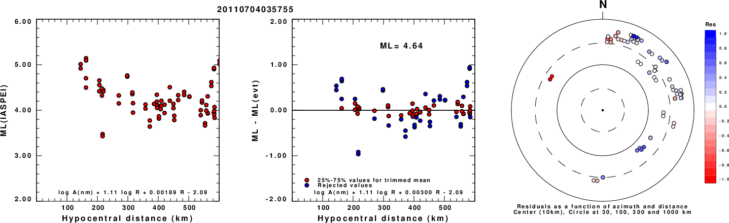
Left: ML computed using the IASPEI formula for Horizontal components. Center: ML residuals computed using a modified IASPEI formula that accounts for path specific attenuation; the values used for the trimmed mean are indicated. The ML relation used for each figure is given at the bottom of each plot.
Right: Residuals from new relation as a function of distance and azimuth.
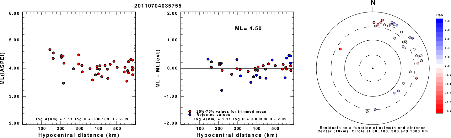
Left: ML computed using the IASPEI formula for Vertical components (research). Center: ML residuals computed using a modified IASPEI formula that accounts for path specific attenuation; the values used for the trimmed mean are indicated. The ML relation used for each figure is given at the bottom of each plot.
Right: Residuals from new relation as a function of distance and azimuth.
Context
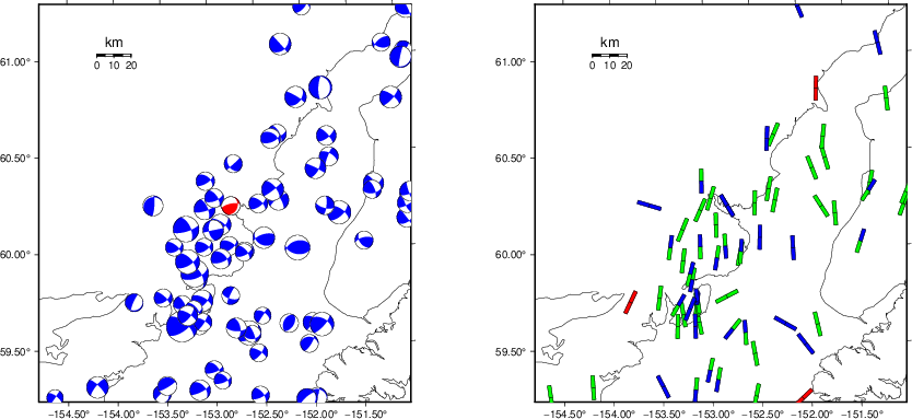
The left panel of the next figure presents the focal mechanism for this earthquake (red) in the context of other nearby events (blue) in the SLU Moment Tensor Catalog. The right panel shows the inferred direction of maximum compressive stress and the type of faulting (green is strike-slip, red is normal, blue is thrust; oblique is shown by a combination of colors). Thus context plot is useful for assessing the appropriateness of the moment tensor of this event.
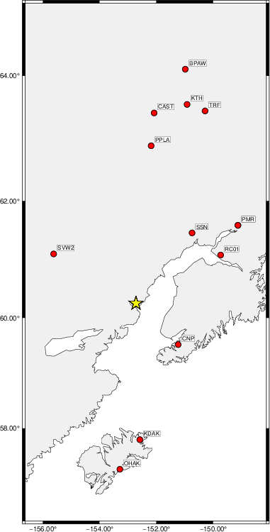
Waveform Inversion using wvfgrd96
The focal mechanism was determined using broadband seismic waveforms. The location of the event (star) and the
stations used for (red) the waveform inversion are shown in the next figure.
|
|
Location of broadband stations used for waveform inversion
|
The program wvfgrd96 was used with good traces observed at short distance to determine the focal mechanism, depth and seismic moment. This technique requires a high quality signal and well determined velocity model for the Green's functions. To the extent that these are the quality data, this type of mechanism should be preferred over the radiation pattern technique which requires the separate step of defining the pressure and tension quadrants and the correct strike.
The observed and predicted traces are filtered using the following gsac commands:
hp c 0.02 n 3
lp c 0.06 n 3
The results of this grid search are as follow:
           DEPTH  STK   DIP  RAKE   MW    FIT
WVFGRD96    0.5    85    50   -70   3.27 0.1748
WVFGRD96    1.0    75    50   -85   3.31 0.1880
WVFGRD96    2.0     5    45   -95   3.39 0.2345
WVFGRD96    3.0   165    45   -95   3.44 0.2554
WVFGRD96    4.0     5    50   -60   3.46 0.2598
WVFGRD96    5.0    20    80     5   3.43 0.2736
WVFGRD96    6.0    20    80     5   3.46 0.2873
WVFGRD96    7.0    20    80     5   3.48 0.3008
WVFGRD96    8.0    20    80     5   3.52 0.3141
WVFGRD96    9.0    20    80    10   3.54 0.3218
WVFGRD96   10.0    20    70   -20   3.54 0.3301
WVFGRD96   11.0   210    70    25   3.54 0.3416
WVFGRD96   12.0   210    70    25   3.56 0.3533
WVFGRD96   13.0   210    70    25   3.57 0.3639
WVFGRD96   14.0   210    70    25   3.58 0.3735
WVFGRD96   15.0   210    70    25   3.60 0.3825
WVFGRD96   16.0   210    70    25   3.61 0.3918
WVFGRD96   17.0   210    70    25   3.62 0.4001
WVFGRD96   18.0   210    70    25   3.63 0.4075
WVFGRD96   19.0   210    70    25   3.64 0.4143
WVFGRD96   20.0   210    70    25   3.65 0.4220
WVFGRD96   21.0   210    70    25   3.66 0.4283
WVFGRD96   22.0   210    75    30   3.68 0.4342
WVFGRD96   23.0   205    70    25   3.71 0.4408
WVFGRD96   24.0   210    75    35   3.71 0.4475
WVFGRD96   25.0   210    75    35   3.72 0.4533
WVFGRD96   26.0   205    75    30   3.74 0.4585
WVFGRD96   27.0   205    75    30   3.75 0.4644
WVFGRD96   28.0   205    75    30   3.76 0.4688
WVFGRD96   29.0   205    75    30   3.77 0.4716
WVFGRD96   30.0   205    75    30   3.78 0.4748
WVFGRD96   31.0   205    75    30   3.79 0.4778
WVFGRD96   32.0   205    75    30   3.80 0.4794
WVFGRD96   33.0   210    75    35   3.80 0.4796
WVFGRD96   34.0   205    75    30   3.82 0.4806
WVFGRD96   35.0   205    75    30   3.83 0.4820
WVFGRD96   36.0   210    75    30   3.82 0.4830
WVFGRD96   37.0   210    75    30   3.83 0.4840
WVFGRD96   38.0   210    80    35   3.85 0.4839
WVFGRD96   39.0   210    75    30   3.86 0.4857
WVFGRD96   40.0   210    75    45   3.95 0.4823
WVFGRD96   41.0   210    75    45   3.96 0.4813
WVFGRD96   42.0   210    75    45   3.97 0.4795
WVFGRD96   43.0   210    75    45   3.98 0.4771
WVFGRD96   44.0   210    75    45   3.99 0.4745
WVFGRD96   45.0   210    75    45   4.00 0.4715
WVFGRD96   46.0   210    75    45   4.00 0.4681
WVFGRD96   47.0   210    75    45   4.01 0.4643
WVFGRD96   48.0   210    75    45   4.02 0.4602
WVFGRD96   49.0   215    70    45   4.01 0.4559
WVFGRD96   50.0   215    70    45   4.01 0.4518
WVFGRD96   51.0   215    70    45   4.02 0.4476
WVFGRD96   52.0   215    70    45   4.02 0.4435
WVFGRD96   53.0   215    70    45   4.03 0.4392
WVFGRD96   54.0   215    70    45   4.03 0.4347
WVFGRD96   55.0   215    70    40   4.02 0.4302
WVFGRD96   56.0   215    70    40   4.02 0.4257
WVFGRD96   57.0    20    70    25   4.03 0.4286
WVFGRD96   58.0    20    70    25   4.04 0.4344
WVFGRD96   59.0    25    65    30   4.03 0.4401
WVFGRD96   60.0    25    65    30   4.03 0.4458
WVFGRD96   61.0    25    65    30   4.03 0.4511
WVFGRD96   62.0    25    65    30   4.04 0.4560
WVFGRD96   63.0    25    65    35   4.06 0.4608
WVFGRD96   64.0    25    65    35   4.06 0.4657
WVFGRD96   65.0    25    65    35   4.06 0.4713
WVFGRD96   66.0    25    65    35   4.07 0.4762
WVFGRD96   67.0    20    65    30   4.09 0.4802
WVFGRD96   68.0    20    65    30   4.09 0.4837
WVFGRD96   69.0    20    65    30   4.09 0.4883
WVFGRD96   70.0    20    65    35   4.11 0.4924
WVFGRD96   71.0    20    65    35   4.11 0.4959
WVFGRD96   72.0    20    65    35   4.11 0.4985
WVFGRD96   73.0    20    65    35   4.12 0.5027
WVFGRD96   74.0    20    65    35   4.12 0.5055
WVFGRD96   75.0    20    65    35   4.12 0.5073
WVFGRD96   76.0    20    65    35   4.12 0.5116
WVFGRD96   77.0    20    65    35   4.12 0.5146
WVFGRD96   78.0    20    65    35   4.12 0.5159
WVFGRD96   79.0    15    45    10   4.10 0.5201
WVFGRD96   80.0    20    40    20   4.09 0.5265
WVFGRD96   81.0    15    40    15   4.12 0.5327
WVFGRD96   82.0    15    40    15   4.12 0.5404
WVFGRD96   83.0    15    40    15   4.12 0.5463
WVFGRD96   84.0    15    40    15   4.12 0.5528
WVFGRD96   85.0    20    35    25   4.12 0.5588
WVFGRD96   86.0    15    40    20   4.14 0.5638
WVFGRD96   87.0    15    40    20   4.15 0.5709
WVFGRD96   88.0    15    35    20   4.15 0.5760
WVFGRD96   89.0    15    35    20   4.15 0.5823
WVFGRD96   90.0    15    35    20   4.15 0.5874
WVFGRD96   91.0    15    35    20   4.15 0.5923
WVFGRD96   92.0    15    35    20   4.15 0.5976
WVFGRD96   93.0    15    35    20   4.16 0.6013
WVFGRD96   94.0    20    35    30   4.16 0.6066
WVFGRD96   95.0    20    35    30   4.16 0.6095
WVFGRD96   96.0    20    30    30   4.16 0.6148
WVFGRD96   97.0    20    30    30   4.17 0.6171
WVFGRD96   98.0    15    35    25   4.18 0.6223
WVFGRD96   99.0    20    30    30   4.17 0.6246
WVFGRD96  100.0    20    30    30   4.17 0.6291
WVFGRD96  101.0    15    35    25   4.18 0.6307
WVFGRD96  102.0    15    35    25   4.18 0.6347
WVFGRD96  103.0    15    35    25   4.18 0.6360
WVFGRD96  104.0    15    35    25   4.19 0.6397
WVFGRD96  105.0    15    35    25   4.19 0.6403
WVFGRD96  106.0    20    30    30   4.17 0.6439
WVFGRD96  107.0    25    30    40   4.18 0.6445
WVFGRD96  108.0    25    30    40   4.19 0.6477
WVFGRD96  109.0    25    30    40   4.19 0.6483
WVFGRD96  110.0    25    30    40   4.19 0.6512
WVFGRD96  111.0    25    30    40   4.19 0.6520
WVFGRD96  112.0    25    30    40   4.19 0.6536
WVFGRD96  113.0    25    30    40   4.19 0.6547
WVFGRD96  114.0    25    30    40   4.19 0.6557
WVFGRD96  115.0    25    30    40   4.19 0.6571
WVFGRD96  116.0    25    30    40   4.19 0.6568
WVFGRD96  117.0    25    30    40   4.19 0.6588
WVFGRD96  118.0    25    30    40   4.19 0.6580
WVFGRD96  119.0    25    30    40   4.19 0.6598
WVFGRD96  120.0    25    30    40   4.19 0.6597
WVFGRD96  121.0    25    30    40   4.19 0.6601
WVFGRD96  122.0    25    30    40   4.19 0.6607
WVFGRD96  123.0    25    30    40   4.19 0.6596
WVFGRD96  124.0    25    30    40   4.19 0.6611
WVFGRD96  125.0    25    30    40   4.19 0.6599
WVFGRD96  126.0    25    30    40   4.19 0.6605
WVFGRD96  127.0    25    30    40   4.20 0.6605
WVFGRD96  128.0    25    30    40   4.20 0.6593
WVFGRD96  129.0    25    30    40   4.20 0.6600
WVFGRD96  130.0    25    30    40   4.20 0.6586
WVFGRD96  131.0    25    30    40   4.20 0.6591
WVFGRD96  132.0    25    30    40   4.20 0.6585
WVFGRD96  133.0    25    30    40   4.20 0.6567
WVFGRD96  134.0    25    30    40   4.20 0.6578
WVFGRD96  135.0    25    30    40   4.20 0.6561
WVFGRD96  136.0    25    30    40   4.20 0.6556
WVFGRD96  137.0    25    30    40   4.20 0.6556
WVFGRD96  138.0    25    30    40   4.20 0.6531
WVFGRD96  139.0    25    30    40   4.20 0.6537
The best solution is
WVFGRD96 124.0 25 30 40 4.19 0.6611
The mechanism corresponding to the best fit is
|
|
Figure 1. Waveform inversion focal mechanism
|
The best fit as a function of depth is given in the following figure:
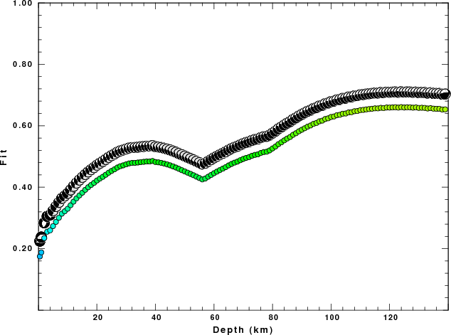
|
|
Figure 2. Depth sensitivity for waveform mechanism
|
The comparison of the observed and predicted waveforms is given in the next figure. The red traces are the observed and the blue are the predicted.
Each observed-predicted component is plotted to the same scale and peak amplitudes are indicated by the numbers to the left of each trace. A pair of numbers is given in black at the right of each predicted traces. The upper number it the time shift required for maximum correlation between the observed and predicted traces. This time shift is required because the synthetics are not computed at exactly the same distance as the observed, the velocity model used in the predictions may not be perfect and the epicentral parameters may be be off.
A positive time shift indicates that the prediction is too fast and should be delayed to match the observed trace (shift to the right in this figure). A negative value indicates that the prediction is too slow. The lower number gives the percentage of variance reduction to characterize the individual goodness of fit (100% indicates a perfect fit).
The bandpass filter used in the processing and for the display was
hp c 0.02 n 3
lp c 0.06 n 3
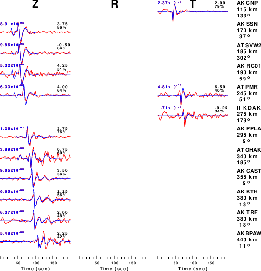
|
|
Figure 3. Waveform comparison for selected depth. Red: observed; Blue - predicted. The time shift with respect to the model prediction is indicated. The percent of fit is also indicated. The time scale is relative to the first trace sample.
|
|
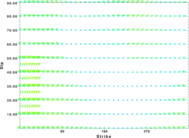
|
Focal mechanism sensitivity at the preferred depth. The red color indicates a very good fit to the waveforms.
Each solution is plotted as a vector at a given value of strike and dip with the angle of the vector representing the rake angle, measured, with respect to the upward vertical (N) in the figure.
|
A check on the assumed source location is possible by looking at the time shifts between the observed and predicted traces. The time shifts for waveform matching arise for several reasons:
- The origin time and epicentral distance are incorrect
- The velocity model used for the inversion is incorrect
- The velocity model used to define the P-arrival time is not the
same as the velocity model used for the waveform inversion
(assuming that the initial trace alignment is based on the
P arrival time)
Assuming only a mislocation, the time shifts are fit to a functional form:
Time_shift = A + B cos Azimuth + C Sin Azimuth
The time shifts for this inversion lead to the next figure:
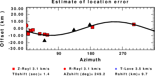
The derived shift in origin time and epicentral coordinates are given at the bottom of the figure.
Velocity Model
The WUS.model used for the waveform synthetic seismograms and for the surface wave eigenfunctions and dispersion is as follows
(The format is in the model96 format of Computer Programs in Seismology).
MODEL.01
Model after     8 iterations
ISOTROPIC
KGS
FLAT EARTH
1-D
CONSTANT VELOCITY
LINE08
LINE09
LINE10
LINE11
      H(KM)   VP(KM/S)   VS(KM/S) RHO(GM/CC)         QP         QS       ETAP       ETAS      FREFP      FREFS
     1.9000     3.4065     2.0089     2.2150  0.302E-02  0.679E-02   0.00       0.00       1.00       1.00
     6.1000     5.5445     3.2953     2.6089  0.349E-02  0.784E-02   0.00       0.00       1.00       1.00
    13.0000     6.2708     3.7396     2.7812  0.212E-02  0.476E-02   0.00       0.00       1.00       1.00
    19.0000     6.4075     3.7680     2.8223  0.111E-02  0.249E-02   0.00       0.00       1.00       1.00
     0.0000     7.9000     4.6200     3.2760  0.164E-10  0.370E-10   0.00       0.00       1.00       1.00
Last Changed Sat Apr 27 02:36:39 PM CDT 2024