Location
Location ANSS
The ANSS event ID is ak0118eu5xs2 and the event page is at
https://earthquake.usgs.gov/earthquakes/eventpage/ak0118eu5xs2/executive.
2011/07/02 11:45:06 63.110 -150.843 122.9 4.3 Alaska
Focal Mechanism
 USGS/SLU Moment Tensor Solution
 ENS  2011/07/02 11:45:06:0  63.11 -150.84 122.9 4.3 Alaska

 Stations used:
   AK.BPAW AK.BRLK AK.CAST AK.CCB AK.DHY AK.FIB AK.KLU AK.KTH
   AK.MCK AK.MLY AK.PPLA AK.RC01 AK.SAW AK.SSN AK.SWD AK.TRF
   AK.WRH AT.PMR IU.COLA

 Filtering commands used:
   hp c 0.02 n 3
   lp c 0.06 n 3

 Best Fitting Double Couple
  Mo = 3.67e+22 dyne-cm
  Mw = 4.31
  Z  = 132 km
  Plane   Strike  Dip  Rake
   NP1       55    75    85
   NP2      254    16   108
  Principal Axes:
   Axis    Value   Plunge  Azimuth
    T   3.67e+22     60     318
    N   0.00e+00      5      56
    P  -3.67e+22     30     149

 Moment Tensor: (dyne-cm)
    Component   Value
       Mxx    -1.52e+22
       Mxy     7.54e+21
       Mxz     2.55e+22
       Myy    -3.11e+21
       Myz    -1.89e+22
       Mzz     1.83e+22


                     --------------
                 ---------#######------
              ------##################----
             ----########################--
           ---##############################-
          ---###############################-#
         --##########   ###################----
        --########### T #################-------
        -############   ###############---------
       --#############################-----------
       -###########################--------------
       -#########################----------------
       -#######################------------------
        ####################--------------------
        #################-----------------------
         #############-------------------------
          #######-----------------   ---------
           ----------------------- P --------
             ---------------------   ------
              ----------------------------
                 ----------------------
                     --------------


 Global CMT Convention Moment Tensor:
      R          T          P
  1.83e+22   2.55e+22   1.89e+22
  2.55e+22  -1.52e+22  -7.54e+21
  1.89e+22  -7.54e+21  -3.11e+21


Details of the solution is found at

http://www.eas.slu.edu/eqc/eqc_mt/MECH.NA/20110702114506/index.html
|
Preferred Solution
The preferred solution from an analysis of the surface-wave spectral amplitude radiation pattern, waveform inversion or first motion observations is
      STK = 55
      DIP = 75
     RAKE = 85
       MW = 4.31
       HS = 132.0
The NDK file is 20110702114506.ndk
The waveform inversion is preferred.
Magnitudes
Given the availability of digital waveforms for determination of the moment tensor, this section documents the added processing leading to mLg, if appropriate to the region, and ML by application of the respective IASPEI formulae. As a research study, the linear distance term of the IASPEI formula
for ML is adjusted to remove a linear distance trend in residuals to give a regionally defined ML. The defined ML uses horizontal component recordings, but the same procedure is applied to the vertical components since there may be some interest in vertical component ground motions. Residual plots versus distance may indicate interesting features of ground motion scaling in some distance ranges. A residual plot of the regionalized magnitude is given as a function of distance and azimuth, since data sets may transcend different wave propagation provinces.
ML Magnitude
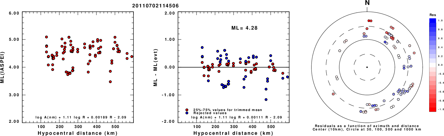
Left: ML computed using the IASPEI formula for Horizontal components. Center: ML residuals computed using a modified IASPEI formula that accounts for path specific attenuation; the values used for the trimmed mean are indicated. The ML relation used for each figure is given at the bottom of each plot.
Right: Residuals from new relation as a function of distance and azimuth.
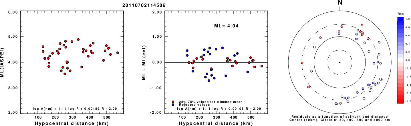
Left: ML computed using the IASPEI formula for Vertical components (research). Center: ML residuals computed using a modified IASPEI formula that accounts for path specific attenuation; the values used for the trimmed mean are indicated. The ML relation used for each figure is given at the bottom of each plot.
Right: Residuals from new relation as a function of distance and azimuth.
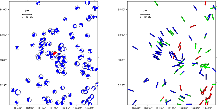
Context
The left panel of the next figure presents the focal mechanism for this earthquake (red) in the context of other nearby events (blue) in the SLU Moment Tensor Catalog. The right panel shows the inferred direction of maximum compressive stress and the type of faulting (green is strike-slip, red is normal, blue is thrust; oblique is shown by a combination of colors). Thus context plot is useful for assessing the appropriateness of the moment tensor of this event.
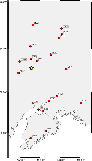
Waveform Inversion using wvfgrd96
The focal mechanism was determined using broadband seismic waveforms. The location of the event (star) and the
stations used for (red) the waveform inversion are shown in the next figure.
|
|
Location of broadband stations used for waveform inversion
|
The program wvfgrd96 was used with good traces observed at short distance to determine the focal mechanism, depth and seismic moment. This technique requires a high quality signal and well determined velocity model for the Green's functions. To the extent that these are the quality data, this type of mechanism should be preferred over the radiation pattern technique which requires the separate step of defining the pressure and tension quadrants and the correct strike.
The observed and predicted traces are filtered using the following gsac commands:
hp c 0.02 n 3
lp c 0.06 n 3
The results of this grid search are as follow:
           DEPTH  STK   DIP  RAKE   MW    FIT
WVFGRD96    0.5   110    40   -70   3.38 0.2149
WVFGRD96    1.0   105    40   -80   3.42 0.2169
WVFGRD96    2.0   115    45   -65   3.52 0.2800
WVFGRD96    3.0   135    50   -40   3.56 0.2894
WVFGRD96    4.0   145    65   -15   3.54 0.2930
WVFGRD96    5.0   335    65    20   3.57 0.3044
WVFGRD96    6.0   335    65    20   3.60 0.3205
WVFGRD96    7.0   335    65    15   3.61 0.3315
WVFGRD96    8.0   340    60    20   3.66 0.3457
WVFGRD96    9.0   340    60    20   3.68 0.3557
WVFGRD96   10.0   340    60    20   3.69 0.3646
WVFGRD96   11.0   340    55    15   3.70 0.3676
WVFGRD96   12.0   340    55    15   3.71 0.3754
WVFGRD96   13.0   340    55    20   3.72 0.3788
WVFGRD96   14.0   340    55    20   3.73 0.3836
WVFGRD96   15.0   340    55    20   3.73 0.3884
WVFGRD96   16.0   340    60    20   3.74 0.3876
WVFGRD96   17.0   340    60    20   3.75 0.3896
WVFGRD96   18.0   340    60    20   3.75 0.3877
WVFGRD96   19.0   345    60    20   3.77 0.3865
WVFGRD96   20.0   345    60    20   3.78 0.3872
WVFGRD96   21.0   230    80   -35   3.76 0.3875
WVFGRD96   22.0   230    80   -35   3.77 0.3900
WVFGRD96   23.0   230    80   -35   3.78 0.3922
WVFGRD96   24.0   230    80   -35   3.78 0.3843
WVFGRD96   25.0   215    85   -35   3.79 0.3877
WVFGRD96   26.0    35    85    30   3.82 0.3912
WVFGRD96   27.0    35    85    30   3.83 0.3946
WVFGRD96   28.0    35    85    30   3.83 0.3881
WVFGRD96   29.0    35    85    30   3.84 0.3932
WVFGRD96   30.0    35    90    30   3.84 0.3970
WVFGRD96   31.0    35    90    30   3.85 0.4022
WVFGRD96   32.0    35    90    30   3.86 0.3957
WVFGRD96   33.0    40    85    30   3.87 0.4006
WVFGRD96   34.0    40    85    30   3.88 0.4053
WVFGRD96   35.0    40    85    30   3.89 0.3994
WVFGRD96   36.0   205    25    60   3.91 0.4070
WVFGRD96   37.0   205    25    60   3.92 0.4166
WVFGRD96   38.0   225    20    85   3.92 0.4162
WVFGRD96   39.0    50    70    90   3.93 0.4266
WVFGRD96   40.0    55    70    95   4.07 0.4413
WVFGRD96   41.0   230    20    90   4.08 0.4367
WVFGRD96   42.0    50    70    90   4.09 0.4389
WVFGRD96   43.0    55    70    95   4.09 0.4402
WVFGRD96   44.0    55    70    95   4.10 0.4399
WVFGRD96   45.0   225    20    85   4.11 0.4391
WVFGRD96   46.0    55    70    95   4.11 0.4350
WVFGRD96   47.0   220    20    80   4.12 0.4325
WVFGRD96   48.0   220    20    80   4.12 0.4296
WVFGRD96   49.0   195    70   -15   4.08 0.4358
WVFGRD96   50.0   195    70   -20   4.08 0.4353
WVFGRD96   51.0   195    70   -20   4.09 0.4408
WVFGRD96   52.0   195    70   -20   4.10 0.4454
WVFGRD96   53.0   195    70   -20   4.10 0.4492
WVFGRD96   54.0   195    70   -20   4.11 0.4523
WVFGRD96   55.0   195    70   -20   4.12 0.4560
WVFGRD96   56.0   195    70   -20   4.12 0.4593
WVFGRD96   57.0   195    70   -20   4.13 0.4628
WVFGRD96   58.0   195    70   -20   4.14 0.4665
WVFGRD96   59.0   195    70   -20   4.14 0.4687
WVFGRD96   60.0   195    70   -20   4.15 0.4721
WVFGRD96   61.0   195    70   -20   4.15 0.4737
WVFGRD96   62.0    55    65    80   4.18 0.4743
WVFGRD96   63.0    55    65    80   4.19 0.4852
WVFGRD96   64.0    55    65    80   4.19 0.4958
WVFGRD96   65.0    55    65    80   4.20 0.5067
WVFGRD96   66.0    60    65    85   4.20 0.5166
WVFGRD96   67.0    60    65    85   4.21 0.5263
WVFGRD96   68.0    60    65    85   4.21 0.5359
WVFGRD96   69.0    55    65    80   4.21 0.5443
WVFGRD96   70.0    55    70    80   4.21 0.5538
WVFGRD96   71.0    55    70    80   4.22 0.5641
WVFGRD96   72.0    55    70    80   4.22 0.5735
WVFGRD96   73.0    55    70    80   4.22 0.5842
WVFGRD96   74.0    55    70    80   4.22 0.5931
WVFGRD96   75.0    55    70    80   4.23 0.6013
WVFGRD96   76.0    55    70    80   4.23 0.6111
WVFGRD96   77.0    55    70    80   4.23 0.6197
WVFGRD96   78.0    55    70    80   4.23 0.6262
WVFGRD96   79.0    55    70    80   4.24 0.6347
WVFGRD96   80.0    55    70    80   4.24 0.6431
WVFGRD96   81.0    55    70    80   4.24 0.6498
WVFGRD96   82.0    55    70    80   4.24 0.6575
WVFGRD96   83.0    55    70    80   4.25 0.6651
WVFGRD96   84.0    55    70    80   4.25 0.6723
WVFGRD96   85.0    55    70    80   4.25 0.6782
WVFGRD96   86.0    55    70    80   4.25 0.6846
WVFGRD96   87.0    55    70    80   4.25 0.6915
WVFGRD96   88.0    55    70    80   4.25 0.6962
WVFGRD96   89.0    55    70    80   4.26 0.7024
WVFGRD96   90.0    55    70    80   4.26 0.7079
WVFGRD96   91.0    55    70    80   4.26 0.7126
WVFGRD96   92.0    55    70    80   4.26 0.7177
WVFGRD96   93.0    55    70    80   4.26 0.7223
WVFGRD96   94.0    55    70    80   4.26 0.7273
WVFGRD96   95.0    55    70    80   4.27 0.7313
WVFGRD96   96.0    55    70    80   4.27 0.7352
WVFGRD96   97.0    55    70    80   4.27 0.7397
WVFGRD96   98.0    55    70    80   4.27 0.7432
WVFGRD96   99.0    55    70    80   4.27 0.7462
WVFGRD96  100.0    55    70    80   4.27 0.7503
WVFGRD96  101.0    55    70    80   4.27 0.7531
WVFGRD96  102.0    55    70    80   4.27 0.7557
WVFGRD96  103.0    55    70    80   4.28 0.7588
WVFGRD96  104.0    55    70    80   4.28 0.7612
WVFGRD96  105.0    55    70    80   4.28 0.7638
WVFGRD96  106.0    55    70    80   4.28 0.7658
WVFGRD96  107.0    55    70    80   4.28 0.7680
WVFGRD96  108.0    55    70    80   4.28 0.7699
WVFGRD96  109.0    55    70    80   4.28 0.7722
WVFGRD96  110.0    55    70    80   4.28 0.7733
WVFGRD96  111.0    55    70    80   4.29 0.7750
WVFGRD96  112.0    55    70    80   4.29 0.7768
WVFGRD96  113.0    55    70    80   4.29 0.7779
WVFGRD96  114.0    55    70    80   4.29 0.7788
WVFGRD96  115.0    55    70    80   4.29 0.7803
WVFGRD96  116.0    55    70    80   4.29 0.7811
WVFGRD96  117.0    55    70    80   4.29 0.7819
WVFGRD96  118.0    55    70    80   4.29 0.7830
WVFGRD96  119.0    55    70    80   4.29 0.7835
WVFGRD96  120.0    55    70    80   4.30 0.7843
WVFGRD96  121.0    55    70    80   4.30 0.7849
WVFGRD96  122.0    55    70    80   4.30 0.7854
WVFGRD96  123.0    55    75    80   4.30 0.7860
WVFGRD96  124.0    55    75    80   4.30 0.7858
WVFGRD96  125.0    55    75    80   4.30 0.7867
WVFGRD96  126.0    55    75    80   4.30 0.7866
WVFGRD96  127.0    55    75    80   4.30 0.7874
WVFGRD96  128.0    55    75    80   4.30 0.7875
WVFGRD96  129.0    55    75    85   4.30 0.7880
WVFGRD96  130.0    55    75    85   4.31 0.7877
WVFGRD96  131.0    55    75    85   4.31 0.7874
WVFGRD96  132.0    55    75    85   4.31 0.7884
WVFGRD96  133.0    55    75    85   4.31 0.7883
WVFGRD96  134.0   260    20   110   4.31 0.7883
WVFGRD96  135.0   260    20   110   4.31 0.7876
WVFGRD96  136.0    55    75    85   4.31 0.7872
WVFGRD96  137.0   260    20   110   4.31 0.7877
WVFGRD96  138.0    55    75    85   4.31 0.7875
WVFGRD96  139.0    55    75    85   4.31 0.7864
The best solution is
WVFGRD96 132.0 55 75 85 4.31 0.7884
The mechanism corresponding to the best fit is
|
|
Figure 1. Waveform inversion focal mechanism
|
The best fit as a function of depth is given in the following figure:
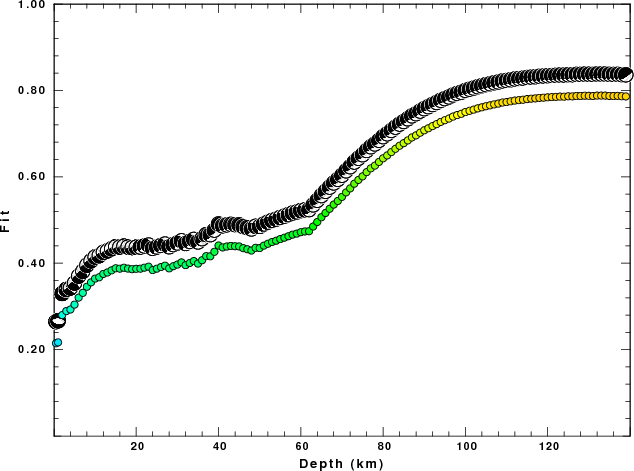
|
|
Figure 2. Depth sensitivity for waveform mechanism
|
The comparison of the observed and predicted waveforms is given in the next figure. The red traces are the observed and the blue are the predicted.
Each observed-predicted component is plotted to the same scale and peak amplitudes are indicated by the numbers to the left of each trace. A pair of numbers is given in black at the right of each predicted traces. The upper number it the time shift required for maximum correlation between the observed and predicted traces. This time shift is required because the synthetics are not computed at exactly the same distance as the observed, the velocity model used in the predictions may not be perfect and the epicentral parameters may be be off.
A positive time shift indicates that the prediction is too fast and should be delayed to match the observed trace (shift to the right in this figure). A negative value indicates that the prediction is too slow. The lower number gives the percentage of variance reduction to characterize the individual goodness of fit (100% indicates a perfect fit).
The bandpass filter used in the processing and for the display was
hp c 0.02 n 3
lp c 0.06 n 3
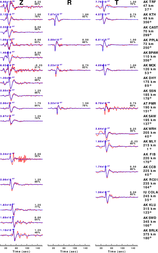
|
|
Figure 3. Waveform comparison for selected depth. Red: observed; Blue - predicted. The time shift with respect to the model prediction is indicated. The percent of fit is also indicated. The time scale is relative to the first trace sample.
|

|
|
Focal mechanism sensitivity at the preferred depth. The red color indicates a very good fit to the waveforms.
Each solution is plotted as a vector at a given value of strike and dip with the angle of the vector representing the rake angle, measured, with respect to the upward vertical (N) in the figure.
|
A check on the assumed source location is possible by looking at the time shifts between the observed and predicted traces. The time shifts for waveform matching arise for several reasons:
- The origin time and epicentral distance are incorrect
- The velocity model used for the inversion is incorrect
- The velocity model used to define the P-arrival time is not the
same as the velocity model used for the waveform inversion
(assuming that the initial trace alignment is based on the
P arrival time)
Assuming only a mislocation, the time shifts are fit to a functional form:
Time_shift = A + B cos Azimuth + C Sin Azimuth
The time shifts for this inversion lead to the next figure:
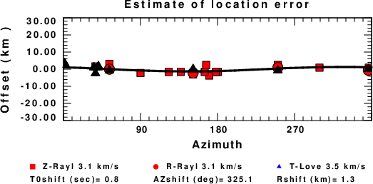
The derived shift in origin time and epicentral coordinates are given at the bottom of the figure.
Velocity Model
The WUS.model used for the waveform synthetic seismograms and for the surface wave eigenfunctions and dispersion is as follows
(The format is in the model96 format of Computer Programs in Seismology).
MODEL.01
Model after     8 iterations
ISOTROPIC
KGS
FLAT EARTH
1-D
CONSTANT VELOCITY
LINE08
LINE09
LINE10
LINE11
      H(KM)   VP(KM/S)   VS(KM/S) RHO(GM/CC)         QP         QS       ETAP       ETAS      FREFP      FREFS
     1.9000     3.4065     2.0089     2.2150  0.302E-02  0.679E-02   0.00       0.00       1.00       1.00
     6.1000     5.5445     3.2953     2.6089  0.349E-02  0.784E-02   0.00       0.00       1.00       1.00
    13.0000     6.2708     3.7396     2.7812  0.212E-02  0.476E-02   0.00       0.00       1.00       1.00
    19.0000     6.4075     3.7680     2.8223  0.111E-02  0.249E-02   0.00       0.00       1.00       1.00
     0.0000     7.9000     4.6200     3.2760  0.164E-10  0.370E-10   0.00       0.00       1.00       1.00
Last Changed Sat Apr 27 02:32:13 PM CDT 2024