Location
Location ANSS
The ANSS event ID is ak0117rtyygs and the event page is at
https://earthquake.usgs.gov/earthquakes/eventpage/ak0117rtyygs/executive.
2011/06/18 20:40:29 62.081 -148.264 29.0 4.5 Alaska
Focal Mechanism
 USGS/SLU Moment Tensor Solution
 ENS  2011/06/18 20:40:29:0  62.08 -148.26  29.0 4.5 Alaska

 Stations used:
   AK.BAL AK.BMR AK.CRQ AK.DIV AK.EYAK AK.KLU AK.MCK AK.MDM
   AK.MLY AK.PAX AK.PPLA AK.RAG AK.SAW AK.SCM AK.SWD AK.TRF
   AT.PMR AT.SVW2 IU.COLA

 Filtering commands used:
   hp c 0.02 n 3
   lp c 0.06 n 3

 Best Fitting Double Couple
  Mo = 1.72e+22 dyne-cm
  Mw = 4.09
  Z  = 46 km
  Plane   Strike  Dip  Rake
   NP1       70    50   -60
   NP2      208    48   -121
  Principal Axes:
   Axis    Value   Plunge  Azimuth
    T   1.72e+22      1     139
    N   0.00e+00     23     230
    P  -1.72e+22     67      47

 Moment Tensor: (dyne-cm)
    Component   Value
       Mxx     8.71e+21
       Mxy    -9.75e+21
       Mxz    -4.32e+21
       Myy     5.94e+21
       Myz    -4.30e+21
       Mzz    -1.47e+22


                     ##############
                 ################------
              ###############-------------
             #############-----------------
           #############---------------------
          ############------------------------
         ############--------------------------
        ############-----------   -------------#
        ###########------------ P -------------#
       ###########-------------   ------------###
       ##########----------------------------####
       #########----------------------------#####
       #########--------------------------#######
        ########------------------------########
        #######----------------------###########
         -#####-------------------#############
          ----##-------------#################
           -----#############################
             ---########################
              ---####################### T
                 -#####################
                     ##############


 Global CMT Convention Moment Tensor:
      R          T          P
 -1.47e+22  -4.32e+21   4.30e+21
 -4.32e+21   8.71e+21   9.75e+21
  4.30e+21   9.75e+21   5.94e+21


Details of the solution is found at

http://www.eas.slu.edu/eqc/eqc_mt/MECH.NA/20110618204029/index.html
|
Preferred Solution
The preferred solution from an analysis of the surface-wave spectral amplitude radiation pattern, waveform inversion or first motion observations is
      STK = 70
      DIP = 50
     RAKE = -60
       MW = 4.09
       HS = 46.0
The NDK file is 20110618204029.ndk
The waveform inversion is preferred.
Magnitudes
Given the availability of digital waveforms for determination of the moment tensor, this section documents the added processing leading to mLg, if appropriate to the region, and ML by application of the respective IASPEI formulae. As a research study, the linear distance term of the IASPEI formula
for ML is adjusted to remove a linear distance trend in residuals to give a regionally defined ML. The defined ML uses horizontal component recordings, but the same procedure is applied to the vertical components since there may be some interest in vertical component ground motions. Residual plots versus distance may indicate interesting features of ground motion scaling in some distance ranges. A residual plot of the regionalized magnitude is given as a function of distance and azimuth, since data sets may transcend different wave propagation provinces.
ML Magnitude
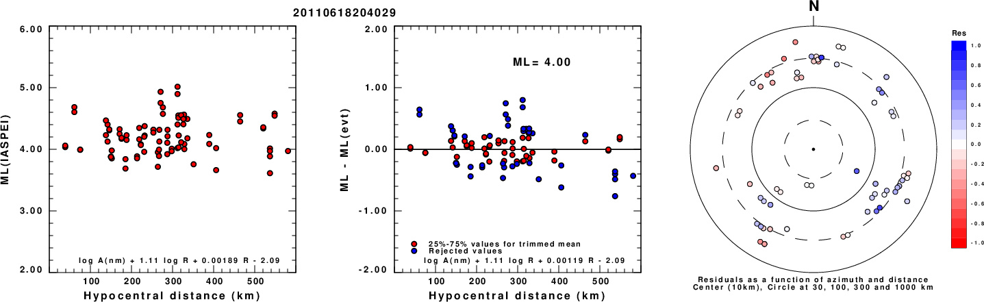
Left: ML computed using the IASPEI formula for Horizontal components. Center: ML residuals computed using a modified IASPEI formula that accounts for path specific attenuation; the values used for the trimmed mean are indicated. The ML relation used for each figure is given at the bottom of each plot.
Right: Residuals from new relation as a function of distance and azimuth.
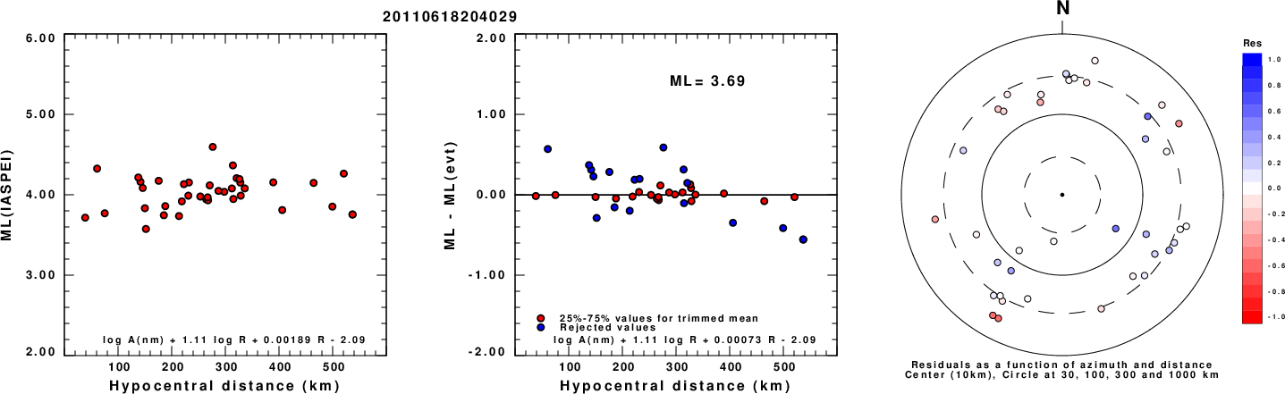
Left: ML computed using the IASPEI formula for Vertical components (research). Center: ML residuals computed using a modified IASPEI formula that accounts for path specific attenuation; the values used for the trimmed mean are indicated. The ML relation used for each figure is given at the bottom of each plot.
Right: Residuals from new relation as a function of distance and azimuth.
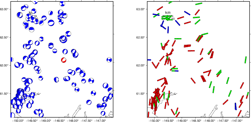
Context
The left panel of the next figure presents the focal mechanism for this earthquake (red) in the context of other nearby events (blue) in the SLU Moment Tensor Catalog. The right panel shows the inferred direction of maximum compressive stress and the type of faulting (green is strike-slip, red is normal, blue is thrust; oblique is shown by a combination of colors). Thus context plot is useful for assessing the appropriateness of the moment tensor of this event.
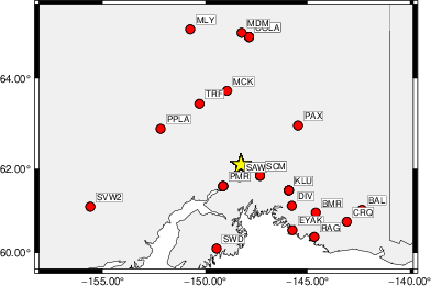
Waveform Inversion using wvfgrd96
The focal mechanism was determined using broadband seismic waveforms. The location of the event (star) and the
stations used for (red) the waveform inversion are shown in the next figure.
|
|
Location of broadband stations used for waveform inversion
|
The program wvfgrd96 was used with good traces observed at short distance to determine the focal mechanism, depth and seismic moment. This technique requires a high quality signal and well determined velocity model for the Green's functions. To the extent that these are the quality data, this type of mechanism should be preferred over the radiation pattern technique which requires the separate step of defining the pressure and tension quadrants and the correct strike.
The observed and predicted traces are filtered using the following gsac commands:
hp c 0.02 n 3
lp c 0.06 n 3
The results of this grid search are as follow:
           DEPTH  STK   DIP  RAKE   MW    FIT
WVFGRD96    0.5   225    45    90   3.37 0.2269
WVFGRD96    1.0    45    45    90   3.41 0.2303
WVFGRD96    2.0    45    45    90   3.52 0.2918
WVFGRD96    3.0   210    45    80   3.61 0.3036
WVFGRD96    4.0   340    90    -5   3.60 0.3076
WVFGRD96    5.0   165    85     0   3.63 0.3042
WVFGRD96    6.0   165    80    -5   3.66 0.2959
WVFGRD96    7.0   165    80    -5   3.68 0.2901
WVFGRD96    8.0   165    75   -10   3.71 0.2869
WVFGRD96    9.0    80    85   -35   3.70 0.2870
WVFGRD96   10.0    90    90   -45   3.68 0.2887
WVFGRD96   11.0   275    80    50   3.69 0.3024
WVFGRD96   12.0   275    80    50   3.71 0.3176
WVFGRD96   13.0   275    80    50   3.72 0.3310
WVFGRD96   14.0   275    80    50   3.73 0.3440
WVFGRD96   15.0    90    90   -50   3.73 0.3573
WVFGRD96   16.0    90    90   -50   3.74 0.3717
WVFGRD96   17.0   270    90    50   3.75 0.3851
WVFGRD96   18.0    85    80   -55   3.74 0.3975
WVFGRD96   19.0    85    80   -50   3.76 0.4116
WVFGRD96   20.0    85    80   -50   3.77 0.4257
WVFGRD96   21.0    85    80   -50   3.79 0.4373
WVFGRD96   22.0    85    75   -55   3.79 0.4503
WVFGRD96   23.0    85    75   -50   3.80 0.4625
WVFGRD96   24.0    80    70   -55   3.80 0.4756
WVFGRD96   25.0    80    70   -55   3.81 0.4880
WVFGRD96   26.0    80    70   -50   3.83 0.4998
WVFGRD96   27.0    80    65   -55   3.83 0.5119
WVFGRD96   28.0    80    65   -55   3.84 0.5238
WVFGRD96   29.0    80    65   -55   3.85 0.5350
WVFGRD96   30.0    80    65   -50   3.86 0.5453
WVFGRD96   31.0    80    65   -50   3.87 0.5547
WVFGRD96   32.0    80    60   -55   3.87 0.5633
WVFGRD96   33.0    80    60   -55   3.88 0.5715
WVFGRD96   34.0    80    60   -55   3.89 0.5790
WVFGRD96   35.0    80    60   -50   3.90 0.5854
WVFGRD96   36.0    75    55   -55   3.91 0.5911
WVFGRD96   37.0    75    55   -55   3.92 0.5971
WVFGRD96   38.0    75    55   -55   3.93 0.6004
WVFGRD96   39.0    70    50   -60   3.95 0.6014
WVFGRD96   40.0    70    55   -60   4.05 0.5948
WVFGRD96   41.0    70    50   -60   4.06 0.6010
WVFGRD96   42.0    70    50   -60   4.06 0.6059
WVFGRD96   43.0    70    50   -60   4.07 0.6104
WVFGRD96   44.0    70    50   -60   4.08 0.6126
WVFGRD96   45.0    70    50   -60   4.09 0.6139
WVFGRD96   46.0    70    50   -60   4.09 0.6139
WVFGRD96   47.0    70    50   -60   4.10 0.6126
WVFGRD96   48.0    70    50   -60   4.10 0.6104
WVFGRD96   49.0    65    45   -65   4.11 0.6079
WVFGRD96   50.0    65    45   -65   4.12 0.6043
WVFGRD96   51.0    65    45   -65   4.12 0.6004
WVFGRD96   52.0    70    45   -60   4.12 0.5955
WVFGRD96   53.0    70    45   -60   4.12 0.5902
WVFGRD96   54.0    70    45   -60   4.13 0.5849
WVFGRD96   55.0    70    45   -60   4.13 0.5784
WVFGRD96   56.0    70    45   -60   4.13 0.5708
WVFGRD96   57.0    70    45   -60   4.14 0.5633
WVFGRD96   58.0    70    45   -60   4.14 0.5547
WVFGRD96   59.0    70    45   -60   4.14 0.5458
The best solution is
WVFGRD96 46.0 70 50 -60 4.09 0.6139
The mechanism corresponding to the best fit is
|
|
Figure 1. Waveform inversion focal mechanism
|
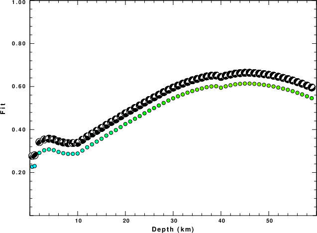
The best fit as a function of depth is given in the following figure:
|
|
Figure 2. Depth sensitivity for waveform mechanism
|
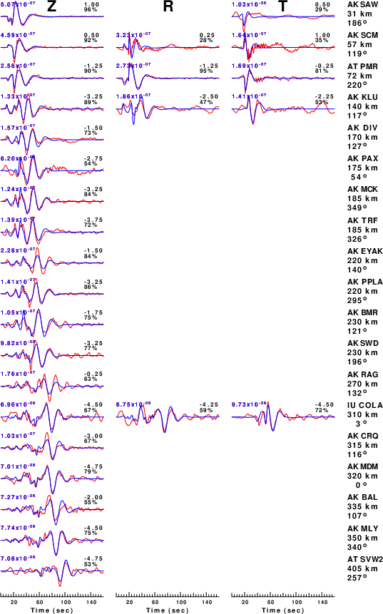
The comparison of the observed and predicted waveforms is given in the next figure. The red traces are the observed and the blue are the predicted.
Each observed-predicted component is plotted to the same scale and peak amplitudes are indicated by the numbers to the left of each trace. A pair of numbers is given in black at the right of each predicted traces. The upper number it the time shift required for maximum correlation between the observed and predicted traces. This time shift is required because the synthetics are not computed at exactly the same distance as the observed, the velocity model used in the predictions may not be perfect and the epicentral parameters may be be off.
A positive time shift indicates that the prediction is too fast and should be delayed to match the observed trace (shift to the right in this figure). A negative value indicates that the prediction is too slow. The lower number gives the percentage of variance reduction to characterize the individual goodness of fit (100% indicates a perfect fit).
The bandpass filter used in the processing and for the display was
hp c 0.02 n 3
lp c 0.06 n 3
|
|
Figure 3. Waveform comparison for selected depth. Red: observed; Blue - predicted. The time shift with respect to the model prediction is indicated. The percent of fit is also indicated. The time scale is relative to the first trace sample.
|
|
|
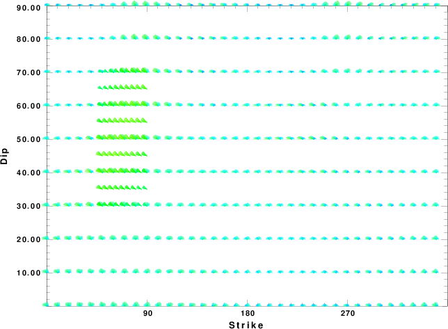
Focal mechanism sensitivity at the preferred depth. The red color indicates a very good fit to the waveforms.
Each solution is plotted as a vector at a given value of strike and dip with the angle of the vector representing the rake angle, measured, with respect to the upward vertical (N) in the figure.
|
A check on the assumed source location is possible by looking at the time shifts between the observed and predicted traces. The time shifts for waveform matching arise for several reasons:
- The origin time and epicentral distance are incorrect
- The velocity model used for the inversion is incorrect
- The velocity model used to define the P-arrival time is not the
same as the velocity model used for the waveform inversion
(assuming that the initial trace alignment is based on the
P arrival time)
Assuming only a mislocation, the time shifts are fit to a functional form:
Time_shift = A + B cos Azimuth + C Sin Azimuth
The time shifts for this inversion lead to the next figure:
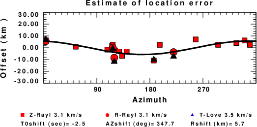
The derived shift in origin time and epicentral coordinates are given at the bottom of the figure.
Velocity Model
The WUS.model used for the waveform synthetic seismograms and for the surface wave eigenfunctions and dispersion is as follows
(The format is in the model96 format of Computer Programs in Seismology).
MODEL.01
Model after     8 iterations
ISOTROPIC
KGS
FLAT EARTH
1-D
CONSTANT VELOCITY
LINE08
LINE09
LINE10
LINE11
      H(KM)   VP(KM/S)   VS(KM/S) RHO(GM/CC)         QP         QS       ETAP       ETAS      FREFP      FREFS
     1.9000     3.4065     2.0089     2.2150  0.302E-02  0.679E-02   0.00       0.00       1.00       1.00
     6.1000     5.5445     3.2953     2.6089  0.349E-02  0.784E-02   0.00       0.00       1.00       1.00
    13.0000     6.2708     3.7396     2.7812  0.212E-02  0.476E-02   0.00       0.00       1.00       1.00
    19.0000     6.4075     3.7680     2.8223  0.111E-02  0.249E-02   0.00       0.00       1.00       1.00
     0.0000     7.9000     4.6200     3.2760  0.164E-10  0.370E-10   0.00       0.00       1.00       1.00
Last Changed Sat Apr 27 02:23:16 PM CDT 2024