Location
Location ANSS
The ANSS event ID is ak0117oi3hnt and the event page is at
https://earthquake.usgs.gov/earthquakes/eventpage/ak0117oi3hnt/executive.
2011/06/16 19:06:05 60.765 -151.076 58.9 5.1 Alaska
Focal Mechanism
 USGS/SLU Moment Tensor Solution
 ENS  2011/06/16 19:06:05:0  60.76 -151.08  58.9 5.1 Alaska

 Stations used:
   AK.BPAW AK.BRLK AK.BWN AK.CNP AK.DIV AK.HOM AK.KLU AK.KTH
   AK.MCK AK.PPLA AK.RC01 AK.RND AK.SAW AK.SCM AK.SSN AK.SWD
   AT.MENT AT.PMR II.KDAK

 Filtering commands used:
   hp c 0.02 n 3
   lp c 0.05 n 3

 Best Fitting Double Couple
  Mo = 3.85e+23 dyne-cm
  Mw = 4.99
  Z  = 74 km
  Plane   Strike  Dip  Rake
   NP1       45    75    20
   NP2      310    71   164
  Principal Axes:
   Axis    Value   Plunge  Azimuth
    T   3.85e+23     25     268
    N   0.00e+00     65      80
    P  -3.85e+23      3     177

 Moment Tensor: (dyne-cm)
    Component   Value
       Mxx    -3.82e+23
       Mxy     3.29e+22
       Mxz     1.44e+22
       Myy     3.16e+23
       Myz    -1.47e+23
       Mzz     6.58e+22


                     --------------
                 ----------------------
              ----------------------------
             -----------------------------#
           ######-------------------------###
          ############-------------------#####
         ################---------------#######
        ####################----------##########
        ######################-------###########
       #########################----#############
       ####   ###################################
       #### T ##################----#############
       ####   #################-------###########
        #####################----------#########
        ###################--------------#######
         ###############------------------#####
          ############---------------------###
           ########-------------------------#
             ###---------------------------
              ----------------------------
                 -----------   --------
                     ------- P ----


 Global CMT Convention Moment Tensor:
      R          T          P
  6.58e+22   1.44e+22   1.47e+23
  1.44e+22  -3.82e+23  -3.29e+22
  1.47e+23  -3.29e+22   3.16e+23


Details of the solution is found at

http://www.eas.slu.edu/eqc/eqc_mt/MECH.NA/20110616190605/index.html
|
Preferred Solution
The preferred solution from an analysis of the surface-wave spectral amplitude radiation pattern, waveform inversion or first motion observations is
      STK = 45
      DIP = 75
     RAKE = 20
       MW = 4.99
       HS = 74.0
The NDK file is 20110616190605.ndk
The waveform inversion is preferred.
Moment Tensor Comparison
The following compares this source inversion to those provided by others. The purpose is to look for major differences and also to note slight differences that might be inherent to the processing procedure. For completeness the USGS/SLU solution is repeated from above.
| SLU |
USGSMT |
 USGS/SLU Moment Tensor Solution
 ENS  2011/06/16 19:06:05:0  60.76 -151.08  58.9 5.1 Alaska

 Stations used:
   AK.BPAW AK.BRLK AK.BWN AK.CNP AK.DIV AK.HOM AK.KLU AK.KTH
   AK.MCK AK.PPLA AK.RC01 AK.RND AK.SAW AK.SCM AK.SSN AK.SWD
   AT.MENT AT.PMR II.KDAK

 Filtering commands used:
   hp c 0.02 n 3
   lp c 0.05 n 3

 Best Fitting Double Couple
  Mo = 3.85e+23 dyne-cm
  Mw = 4.99
  Z  = 74 km
  Plane   Strike  Dip  Rake
   NP1       45    75    20
   NP2      310    71   164
  Principal Axes:
   Axis    Value   Plunge  Azimuth
    T   3.85e+23     25     268
    N   0.00e+00     65      80
    P  -3.85e+23      3     177

 Moment Tensor: (dyne-cm)
    Component   Value
       Mxx    -3.82e+23
       Mxy     3.29e+22
       Mxz     1.44e+22
       Myy     3.16e+23
       Myz    -1.47e+23
       Mzz     6.58e+22


                     --------------
                 ----------------------
              ----------------------------
             -----------------------------#
           ######-------------------------###
          ############-------------------#####
         ################---------------#######
        ####################----------##########
        ######################-------###########
       #########################----#############
       ####   ###################################
       #### T ##################----#############
       ####   #################-------###########
        #####################----------#########
        ###################--------------#######
         ###############------------------#####
          ############---------------------###
           ########-------------------------#
             ###---------------------------
              ----------------------------
                 -----------   --------
                     ------- P ----


 Global CMT Convention Moment Tensor:
      R          T          P
  6.58e+22   1.44e+22   1.47e+23
  1.44e+22  -3.82e+23  -3.29e+22
  1.47e+23  -3.29e+22   3.16e+23


Details of the solution is found at

http://www.eas.slu.edu/eqc/eqc_mt/MECH.NA/20110616190605/index.html
|
USGS/SLU Regional Moment Solution

11/06/16 19:06:05.42

Epicenter:  60.807 -151.216
MW 5.0

USGS/SLU REGIONAL MOMENT TENSOR
Depth  66         No. of sta: 58
Moment Tensor;   Scale 10**16 Nm
  Mrr= 0.17       Mtt=-3.62
  Mpp= 3.45       Mrt= 0.40
  Mrp= 1.31       Mtp=-0.15
 Principal axes:
  T  Val=  3.91  Plg=19  Azm=270
  N       -0.23      69       69
  P       -3.68       7      177

Best Double Couple:Mo=3.8*10**16
 NP1:Strike= 45 Dip=81 Slip=  19
 NP2:       312     71       171
|
Magnitudes
Given the availability of digital waveforms for determination of the moment tensor, this section documents the added processing leading to mLg, if appropriate to the region, and ML by application of the respective IASPEI formulae. As a research study, the linear distance term of the IASPEI formula
for ML is adjusted to remove a linear distance trend in residuals to give a regionally defined ML. The defined ML uses horizontal component recordings, but the same procedure is applied to the vertical components since there may be some interest in vertical component ground motions. Residual plots versus distance may indicate interesting features of ground motion scaling in some distance ranges. A residual plot of the regionalized magnitude is given as a function of distance and azimuth, since data sets may transcend different wave propagation provinces.
ML Magnitude
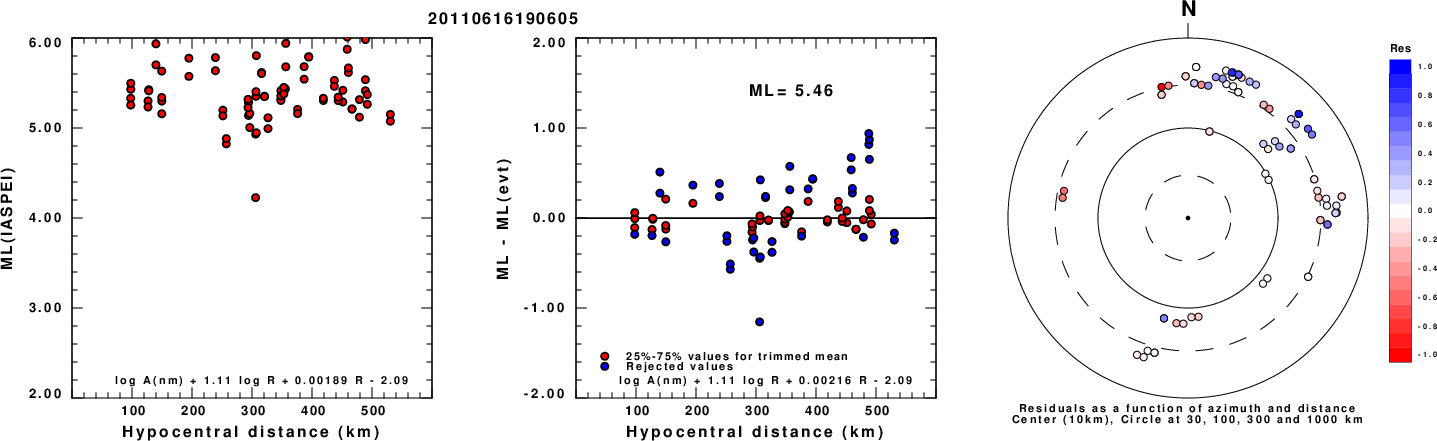
Left: ML computed using the IASPEI formula for Horizontal components. Center: ML residuals computed using a modified IASPEI formula that accounts for path specific attenuation; the values used for the trimmed mean are indicated. The ML relation used for each figure is given at the bottom of each plot.
Right: Residuals from new relation as a function of distance and azimuth.
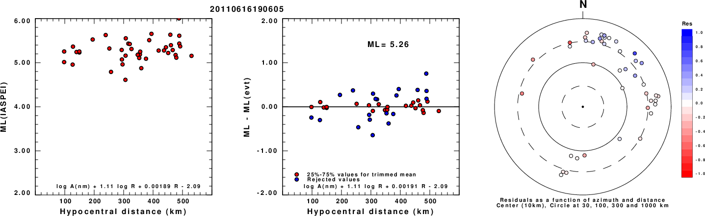
Left: ML computed using the IASPEI formula for Vertical components (research). Center: ML residuals computed using a modified IASPEI formula that accounts for path specific attenuation; the values used for the trimmed mean are indicated. The ML relation used for each figure is given at the bottom of each plot.
Right: Residuals from new relation as a function of distance and azimuth.
Context
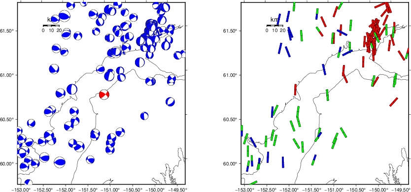
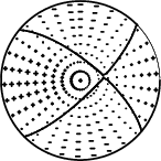
The left panel of the next figure presents the focal mechanism for this earthquake (red) in the context of other nearby events (blue) in the SLU Moment Tensor Catalog. The right panel shows the inferred direction of maximum compressive stress and the type of faulting (green is strike-slip, red is normal, blue is thrust; oblique is shown by a combination of colors). Thus context plot is useful for assessing the appropriateness of the moment tensor of this event.
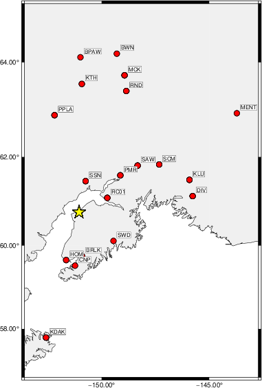
Waveform Inversion using wvfgrd96
The focal mechanism was determined using broadband seismic waveforms. The location of the event (star) and the
stations used for (red) the waveform inversion are shown in the next figure.
|
|
Location of broadband stations used for waveform inversion
|
The program wvfgrd96 was used with good traces observed at short distance to determine the focal mechanism, depth and seismic moment. This technique requires a high quality signal and well determined velocity model for the Green's functions. To the extent that these are the quality data, this type of mechanism should be preferred over the radiation pattern technique which requires the separate step of defining the pressure and tension quadrants and the correct strike.
The observed and predicted traces are filtered using the following gsac commands:
hp c 0.02 n 3
lp c 0.05 n 3
The results of this grid search are as follow:
           DEPTH  STK   DIP  RAKE   MW    FIT
WVFGRD96    0.5   315    70    15   4.16 0.2135
WVFGRD96    1.0   310    85     0   4.17 0.2327
WVFGRD96    2.0   315    75    15   4.28 0.2936
WVFGRD96    3.0   130    90     0   4.31 0.3231
WVFGRD96    4.0   310    85     0   4.34 0.3426
WVFGRD96    5.0   220    80    15   4.38 0.3572
WVFGRD96    6.0   220    80    15   4.41 0.3817
WVFGRD96    7.0    35    90    -5   4.44 0.4075
WVFGRD96    8.0   220    85    15   4.47 0.4351
WVFGRD96    9.0   220    85    15   4.49 0.4546
WVFGRD96   10.0   220    85    15   4.51 0.4696
WVFGRD96   11.0    40    90   -10   4.52 0.4766
WVFGRD96   12.0    35    90   -15   4.54 0.4838
WVFGRD96   13.0    35    90   -15   4.55 0.4888
WVFGRD96   14.0    35    90   -10   4.56 0.4933
WVFGRD96   15.0    35    90   -10   4.57 0.4974
WVFGRD96   16.0    35    90   -15   4.58 0.5003
WVFGRD96   17.0    35    90   -10   4.58 0.5031
WVFGRD96   18.0    35    90   -10   4.59 0.5060
WVFGRD96   19.0    35    90   -10   4.60 0.5088
WVFGRD96   20.0    35    90   -10   4.61 0.5121
WVFGRD96   21.0    35    90   -10   4.61 0.5162
WVFGRD96   22.0    35    90   -10   4.62 0.5192
WVFGRD96   23.0    35    90   -10   4.63 0.5219
WVFGRD96   24.0   215    90    10   4.64 0.5242
WVFGRD96   25.0    35    90   -10   4.64 0.5267
WVFGRD96   26.0    40    90    10   4.64 0.5291
WVFGRD96   27.0    40    90    10   4.65 0.5327
WVFGRD96   28.0    40    90    10   4.66 0.5370
WVFGRD96   29.0   215    85   -15   4.67 0.5433
WVFGRD96   30.0   215    85   -15   4.67 0.5485
WVFGRD96   31.0   215    85   -15   4.68 0.5533
WVFGRD96   32.0   215    85   -15   4.69 0.5583
WVFGRD96   33.0    40    85    10   4.71 0.5669
WVFGRD96   34.0    40    85    10   4.72 0.5748
WVFGRD96   35.0   220    90   -10   4.73 0.5779
WVFGRD96   36.0    40    85    10   4.74 0.5916
WVFGRD96   37.0   220    90   -10   4.76 0.5931
WVFGRD96   38.0    40    85    10   4.77 0.6092
WVFGRD96   39.0    40    85    10   4.79 0.6184
WVFGRD96   40.0    40    80    20   4.82 0.6262
WVFGRD96   41.0    40    80    15   4.83 0.6302
WVFGRD96   42.0    40    80    15   4.83 0.6343
WVFGRD96   43.0    40    80    15   4.84 0.6382
WVFGRD96   44.0    40    80    15   4.85 0.6422
WVFGRD96   45.0    40    80    15   4.86 0.6460
WVFGRD96   46.0    40    80    15   4.86 0.6497
WVFGRD96   47.0    40    80    15   4.87 0.6536
WVFGRD96   48.0    40    80    15   4.88 0.6576
WVFGRD96   49.0    40    80    15   4.88 0.6618
WVFGRD96   50.0    40    80    15   4.89 0.6656
WVFGRD96   51.0    40    80    15   4.90 0.6690
WVFGRD96   52.0    40    80    15   4.90 0.6729
WVFGRD96   53.0    40    80    15   4.91 0.6771
WVFGRD96   54.0    40    80    15   4.91 0.6803
WVFGRD96   55.0    40    80    15   4.92 0.6830
WVFGRD96   56.0    40    80    15   4.93 0.6868
WVFGRD96   57.0    40    80    15   4.93 0.6900
WVFGRD96   58.0    40    80    15   4.93 0.6921
WVFGRD96   59.0    40    80    15   4.94 0.6953
WVFGRD96   60.0    40    80    20   4.94 0.6978
WVFGRD96   61.0    45    75    20   4.95 0.6994
WVFGRD96   62.0    45    75    20   4.95 0.7026
WVFGRD96   63.0    45    75    20   4.95 0.7044
WVFGRD96   64.0    45    75    20   4.96 0.7063
WVFGRD96   65.0    45    75    20   4.96 0.7085
WVFGRD96   66.0    45    75    20   4.96 0.7091
WVFGRD96   67.0    45    75    20   4.97 0.7113
WVFGRD96   68.0    45    75    20   4.97 0.7118
WVFGRD96   69.0    45    75    20   4.97 0.7131
WVFGRD96   70.0    45    75    20   4.98 0.7140
WVFGRD96   71.0    45    75    20   4.98 0.7143
WVFGRD96   72.0    45    75    20   4.98 0.7150
WVFGRD96   73.0    45    75    20   4.98 0.7145
WVFGRD96   74.0    45    75    20   4.99 0.7151
WVFGRD96   75.0    45    75    20   4.99 0.7144
WVFGRD96   76.0    45    75    20   4.99 0.7150
WVFGRD96   77.0    45    75    20   4.99 0.7138
WVFGRD96   78.0    45    75    20   5.00 0.7139
WVFGRD96   79.0    45    75    20   5.00 0.7127
WVFGRD96   80.0    45    75    20   5.00 0.7128
WVFGRD96   81.0    45    75    20   5.00 0.7111
WVFGRD96   82.0    45    75    20   5.00 0.7106
WVFGRD96   83.0    45    75    20   5.01 0.7094
WVFGRD96   84.0    45    75    20   5.01 0.7083
WVFGRD96   85.0    45    75    20   5.01 0.7067
WVFGRD96   86.0    45    75    20   5.01 0.7056
WVFGRD96   87.0    45    75    20   5.01 0.7043
WVFGRD96   88.0    45    75    20   5.01 0.7018
WVFGRD96   89.0    45    75    20   5.02 0.7012
WVFGRD96   90.0    40    80    20   5.02 0.6987
WVFGRD96   91.0    40    80    20   5.02 0.6978
WVFGRD96   92.0    40    80    20   5.02 0.6963
WVFGRD96   93.0    40    80    20   5.02 0.6944
WVFGRD96   94.0    40    80    25   5.02 0.6932
WVFGRD96   95.0    40    80    25   5.02 0.6911
WVFGRD96   96.0    40    80    25   5.02 0.6900
WVFGRD96   97.0    40    80    25   5.02 0.6883
WVFGRD96   98.0    40    80    25   5.02 0.6867
WVFGRD96   99.0    40    80    25   5.02 0.6847
The best solution is
WVFGRD96 74.0 45 75 20 4.99 0.7151
The mechanism corresponding to the best fit is
|
|
Figure 1. Waveform inversion focal mechanism
|
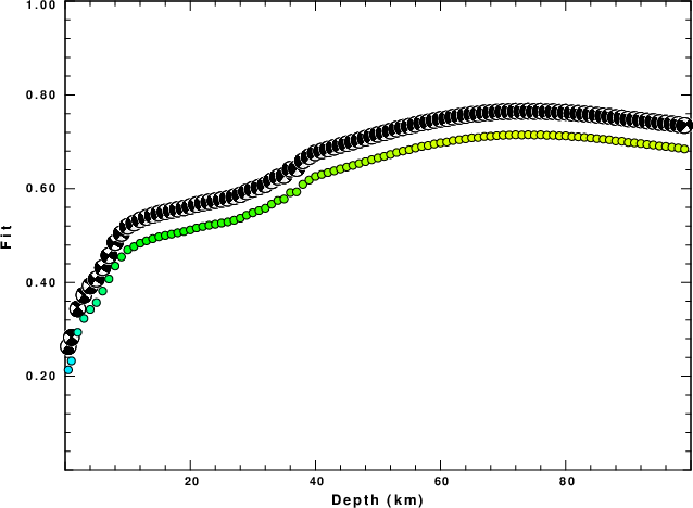
The best fit as a function of depth is given in the following figure:
|
|
Figure 2. Depth sensitivity for waveform mechanism
|
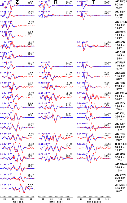
The comparison of the observed and predicted waveforms is given in the next figure. The red traces are the observed and the blue are the predicted.
Each observed-predicted component is plotted to the same scale and peak amplitudes are indicated by the numbers to the left of each trace. A pair of numbers is given in black at the right of each predicted traces. The upper number it the time shift required for maximum correlation between the observed and predicted traces. This time shift is required because the synthetics are not computed at exactly the same distance as the observed, the velocity model used in the predictions may not be perfect and the epicentral parameters may be be off.
A positive time shift indicates that the prediction is too fast and should be delayed to match the observed trace (shift to the right in this figure). A negative value indicates that the prediction is too slow. The lower number gives the percentage of variance reduction to characterize the individual goodness of fit (100% indicates a perfect fit).
The bandpass filter used in the processing and for the display was
hp c 0.02 n 3
lp c 0.05 n 3
|
|
Figure 3. Waveform comparison for selected depth. Red: observed; Blue - predicted. The time shift with respect to the model prediction is indicated. The percent of fit is also indicated. The time scale is relative to the first trace sample.
|
|
|
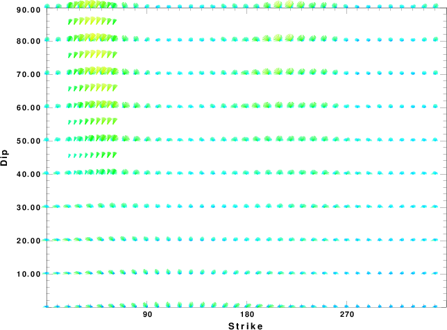
Focal mechanism sensitivity at the preferred depth. The red color indicates a very good fit to the waveforms.
Each solution is plotted as a vector at a given value of strike and dip with the angle of the vector representing the rake angle, measured, with respect to the upward vertical (N) in the figure.
|
A check on the assumed source location is possible by looking at the time shifts between the observed and predicted traces. The time shifts for waveform matching arise for several reasons:
- The origin time and epicentral distance are incorrect
- The velocity model used for the inversion is incorrect
- The velocity model used to define the P-arrival time is not the
same as the velocity model used for the waveform inversion
(assuming that the initial trace alignment is based on the
P arrival time)
Assuming only a mislocation, the time shifts are fit to a functional form:
Time_shift = A + B cos Azimuth + C Sin Azimuth
The time shifts for this inversion lead to the next figure:
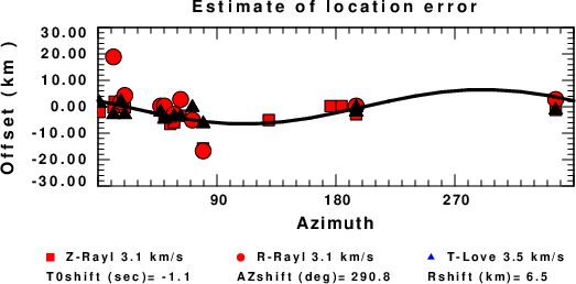
The derived shift in origin time and epicentral coordinates are given at the bottom of the figure.
Velocity Model
The WUS.model used for the waveform synthetic seismograms and for the surface wave eigenfunctions and dispersion is as follows
(The format is in the model96 format of Computer Programs in Seismology).
MODEL.01
Model after     8 iterations
ISOTROPIC
KGS
FLAT EARTH
1-D
CONSTANT VELOCITY
LINE08
LINE09
LINE10
LINE11
      H(KM)   VP(KM/S)   VS(KM/S) RHO(GM/CC)         QP         QS       ETAP       ETAS      FREFP      FREFS
     1.9000     3.4065     2.0089     2.2150  0.302E-02  0.679E-02   0.00       0.00       1.00       1.00
     6.1000     5.5445     3.2953     2.6089  0.349E-02  0.784E-02   0.00       0.00       1.00       1.00
    13.0000     6.2708     3.7396     2.7812  0.212E-02  0.476E-02   0.00       0.00       1.00       1.00
    19.0000     6.4075     3.7680     2.8223  0.111E-02  0.249E-02   0.00       0.00       1.00       1.00
     0.0000     7.9000     4.6200     3.2760  0.164E-10  0.370E-10   0.00       0.00       1.00       1.00
Last Changed Sat Apr 27 02:19:33 PM CDT 2024