Location
Location ANSS
The ANSS event ID is ak0115aiaea0 and the event page is at
https://earthquake.usgs.gov/earthquakes/eventpage/ak0115aiaea0/executive.
2011/04/25 19:29:15 59.062 -152.532 57.4 5 Alaska
Focal Mechanism
 USGS/SLU Moment Tensor Solution
 ENS  2011/04/25 19:29:15:0  59.06 -152.53  57.4 5.0 Alaska

 Stations used:
   AK.BMR AK.BPAW AK.BRLK AK.CAST AK.DHY AK.DIV AK.HOM AK.KLU
   AK.KTH AK.SAW AK.SCM AK.SWD AT.OHAK AT.PMR AT.SVW2 AT.TTA
   II.KDAK

 Filtering commands used:
   hp c 0.02 n 3
   lp c 0.10 n 3

 Best Fitting Double Couple
  Mo = 3.47e+23 dyne-cm
  Mw = 4.96
  Z  = 63 km
  Plane   Strike  Dip  Rake
   NP1      324    67   153
   NP2       65    65    25
  Principal Axes:
   Axis    Value   Plunge  Azimuth
    T   3.47e+23     35     284
    N   0.00e+00     55     107
    P  -3.47e+23      2      15

 Moment Tensor: (dyne-cm)
    Component   Value
       Mxx    -3.10e+23
       Mxy    -1.40e+23
       Mxz     2.92e+22
       Myy     1.98e+23
       Myz    -1.60e+23
       Mzz     1.12e+23


                     ----------- P
                 ---------------   ----
              #####-----------------------
             #########---------------------
           ##############--------------------
          #################-------------------
         ####################------------------
        ######################----------------##
        #####   ################------------####
       ###### T #################----------######
       ######   ##################-------########
       ############################----##########
       ##########################################
        #########################----###########
        #####################---------##########
         ###############---------------########
          -----------------------------#######
           -----------------------------#####
             ---------------------------###
              --------------------------##
                 ----------------------
                     --------------


 Global CMT Convention Moment Tensor:
      R          T          P
  1.12e+23   2.92e+22   1.60e+23
  2.92e+22  -3.10e+23   1.40e+23
  1.60e+23   1.40e+23   1.98e+23


Details of the solution is found at

http://www.eas.slu.edu/eqc/eqc_mt/MECH.NA/20110425192915/index.html
|
Preferred Solution
The preferred solution from an analysis of the surface-wave spectral amplitude radiation pattern, waveform inversion or first motion observations is
      STK = 65
      DIP = 65
     RAKE = 25
       MW = 4.96
       HS = 63.0
The NDK file is 20110425192915.ndk
The waveform inversion is preferred.
Moment Tensor Comparison
The following compares this source inversion to those provided by others. The purpose is to look for major differences and also to note slight differences that might be inherent to the processing procedure. For completeness the USGS/SLU solution is repeated from above.
| SLU |
USGSMT |
 USGS/SLU Moment Tensor Solution
 ENS  2011/04/25 19:29:15:0  59.06 -152.53  57.4 5.0 Alaska

 Stations used:
   AK.BMR AK.BPAW AK.BRLK AK.CAST AK.DHY AK.DIV AK.HOM AK.KLU
   AK.KTH AK.SAW AK.SCM AK.SWD AT.OHAK AT.PMR AT.SVW2 AT.TTA
   II.KDAK

 Filtering commands used:
   hp c 0.02 n 3
   lp c 0.10 n 3

 Best Fitting Double Couple
  Mo = 3.47e+23 dyne-cm
  Mw = 4.96
  Z  = 63 km
  Plane   Strike  Dip  Rake
   NP1      324    67   153
   NP2       65    65    25
  Principal Axes:
   Axis    Value   Plunge  Azimuth
    T   3.47e+23     35     284
    N   0.00e+00     55     107
    P  -3.47e+23      2      15

 Moment Tensor: (dyne-cm)
    Component   Value
       Mxx    -3.10e+23
       Mxy    -1.40e+23
       Mxz     2.92e+22
       Myy     1.98e+23
       Myz    -1.60e+23
       Mzz     1.12e+23


                     ----------- P
                 ---------------   ----
              #####-----------------------
             #########---------------------
           ##############--------------------
          #################-------------------
         ####################------------------
        ######################----------------##
        #####   ################------------####
       ###### T #################----------######
       ######   ##################-------########
       ############################----##########
       ##########################################
        #########################----###########
        #####################---------##########
         ###############---------------########
          -----------------------------#######
           -----------------------------#####
             ---------------------------###
              --------------------------##
                 ----------------------
                     --------------


 Global CMT Convention Moment Tensor:
      R          T          P
  1.12e+23   2.92e+22   1.60e+23
  2.92e+22  -3.10e+23   1.40e+23
  1.60e+23   1.40e+23   1.98e+23


Details of the solution is found at

http://www.eas.slu.edu/eqc/eqc_mt/MECH.NA/20110425192915/index.html
|
USGS/SLU Regional Moment Solution

11/04/25 19:29:15.59

Epicenter:  59.175 -152.834
MW 4.9

USGS/SLU REGIONAL MOMENT TENSOR
Depth  56         No. of sta: 43
Moment Tensor;   Scale 10**16 Nm
  Mrr= 0.48       Mtt=-1.79
  Mpp= 1.31       Mrt= 0.67
  Mrp= 0.78       Mtp= 2.14
 Principal axes:
  T  Val=  2.83  Plg=23  Azm=298
  N        0.07      66      106
  P       -2.90       4      206

Best Double Couple:Mo=2.9*10**16
 NP1:Strike= 74 Dip=77 Slip=  20
 NP2:       340     71       166

|
|
|
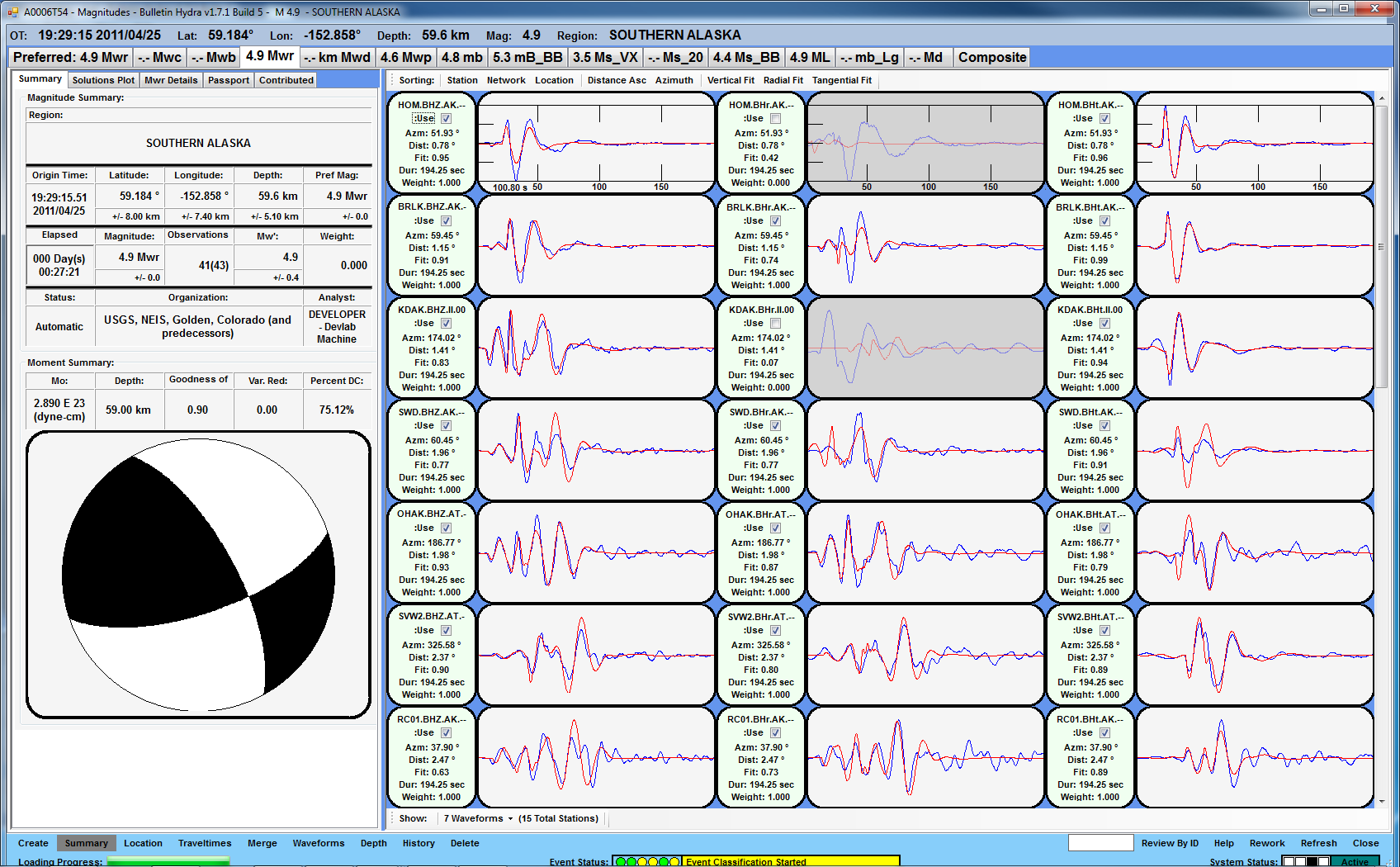
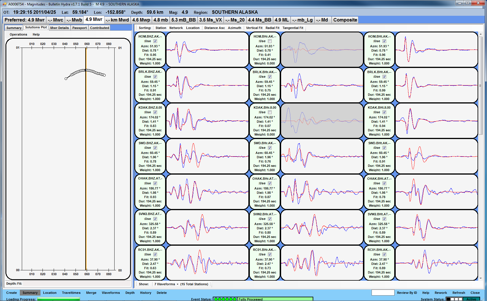
Magnitudes
Given the availability of digital waveforms for determination of the moment tensor, this section documents the added processing leading to mLg, if appropriate to the region, and ML by application of the respective IASPEI formulae. As a research study, the linear distance term of the IASPEI formula
for ML is adjusted to remove a linear distance trend in residuals to give a regionally defined ML. The defined ML uses horizontal component recordings, but the same procedure is applied to the vertical components since there may be some interest in vertical component ground motions. Residual plots versus distance may indicate interesting features of ground motion scaling in some distance ranges. A residual plot of the regionalized magnitude is given as a function of distance and azimuth, since data sets may transcend different wave propagation provinces.
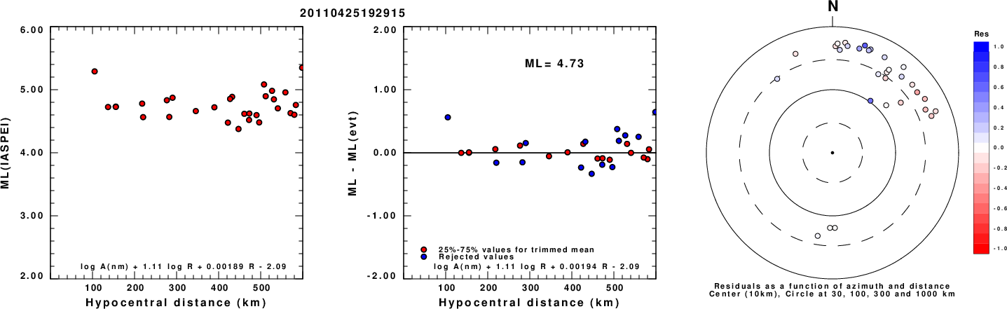
ML Magnitude
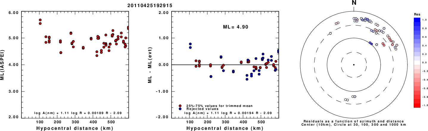
Left: ML computed using the IASPEI formula for Horizontal components. Center: ML residuals computed using a modified IASPEI formula that accounts for path specific attenuation; the values used for the trimmed mean are indicated. The ML relation used for each figure is given at the bottom of each plot.
Right: Residuals from new relation as a function of distance and azimuth.
Left: ML computed using the IASPEI formula for Vertical components (research). Center: ML residuals computed using a modified IASPEI formula that accounts for path specific attenuation; the values used for the trimmed mean are indicated. The ML relation used for each figure is given at the bottom of each plot.
Right: Residuals from new relation as a function of distance and azimuth.
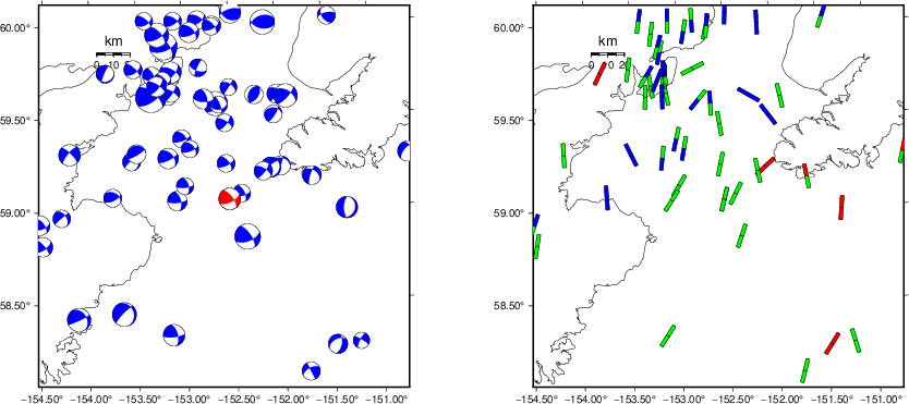
Context
The left panel of the next figure presents the focal mechanism for this earthquake (red) in the context of other nearby events (blue) in the SLU Moment Tensor Catalog. The right panel shows the inferred direction of maximum compressive stress and the type of faulting (green is strike-slip, red is normal, blue is thrust; oblique is shown by a combination of colors). Thus context plot is useful for assessing the appropriateness of the moment tensor of this event.
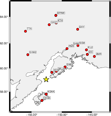
Waveform Inversion using wvfgrd96
The focal mechanism was determined using broadband seismic waveforms. The location of the event (star) and the
stations used for (red) the waveform inversion are shown in the next figure.
|
|
Location of broadband stations used for waveform inversion
|
The program wvfgrd96 was used with good traces observed at short distance to determine the focal mechanism, depth and seismic moment. This technique requires a high quality signal and well determined velocity model for the Green's functions. To the extent that these are the quality data, this type of mechanism should be preferred over the radiation pattern technique which requires the separate step of defining the pressure and tension quadrants and the correct strike.
The observed and predicted traces are filtered using the following gsac commands:
hp c 0.02 n 3
lp c 0.10 n 3
The results of this grid search are as follow:
           DEPTH  STK   DIP  RAKE   MW    FIT
WVFGRD96    0.5   320    50   -30   4.01 0.2262
WVFGRD96    1.0   330    70   -15   4.00 0.2270
WVFGRD96    2.0   330    80   -10   4.13 0.2885
WVFGRD96    3.0   320    85   -45   4.24 0.3318
WVFGRD96    4.0   325    90   -35   4.25 0.3588
WVFGRD96    5.0   325    90   -30   4.28 0.3732
WVFGRD96    6.0   325    90   -30   4.30 0.3797
WVFGRD96    7.0   325    90   -25   4.33 0.3827
WVFGRD96    8.0   325    90   -30   4.37 0.3810
WVFGRD96    9.0   300    75   -25   4.39 0.3817
WVFGRD96   10.0   300    75   -25   4.41 0.3797
WVFGRD96   11.0   300    70   -25   4.44 0.3766
WVFGRD96   12.0   300    70   -25   4.45 0.3728
WVFGRD96   13.0   300    70   -25   4.47 0.3671
WVFGRD96   14.0   300    70   -25   4.48 0.3598
WVFGRD96   15.0   300    70   -25   4.49 0.3509
WVFGRD96   16.0   300    70   -25   4.50 0.3403
WVFGRD96   17.0   300    70   -25   4.51 0.3293
WVFGRD96   18.0   240    65    10   4.51 0.3219
WVFGRD96   19.0   240    65    10   4.53 0.3262
WVFGRD96   20.0   240    65    10   4.54 0.3307
WVFGRD96   21.0   235    65    10   4.55 0.3362
WVFGRD96   22.0   235    65     5   4.57 0.3443
WVFGRD96   23.0   235    65     0   4.58 0.3547
WVFGRD96   24.0   235    65     0   4.59 0.3642
WVFGRD96   25.0   235    65     0   4.61 0.3747
WVFGRD96   26.0   240    75    15   4.62 0.3867
WVFGRD96   27.0   240    75    15   4.64 0.4058
WVFGRD96   28.0   240    70    15   4.64 0.4248
WVFGRD96   29.0   240    70    15   4.66 0.4433
WVFGRD96   30.0   240    70    15   4.67 0.4597
WVFGRD96   31.0   240    70    15   4.68 0.4756
WVFGRD96   32.0   240    70    15   4.69 0.4907
WVFGRD96   33.0   240    75    10   4.70 0.5037
WVFGRD96   34.0   240    75    10   4.71 0.5139
WVFGRD96   35.0   240    75    10   4.72 0.5247
WVFGRD96   36.0   240    75    10   4.74 0.5346
WVFGRD96   37.0   240    75    10   4.75 0.5433
WVFGRD96   38.0    60    85     0   4.78 0.5544
WVFGRD96   39.0    60    85     0   4.80 0.5697
WVFGRD96   40.0    65    75    10   4.84 0.5842
WVFGRD96   41.0    65    75    10   4.86 0.5866
WVFGRD96   42.0    65    75    10   4.87 0.5867
WVFGRD96   43.0    65    75    10   4.88 0.5887
WVFGRD96   44.0    65    70    15   4.89 0.5929
WVFGRD96   45.0    65    70    15   4.90 0.5996
WVFGRD96   46.0    65    70    15   4.91 0.6074
WVFGRD96   47.0    65    70    15   4.92 0.6165
WVFGRD96   48.0    65    70    15   4.93 0.6253
WVFGRD96   49.0    65    70    15   4.93 0.6339
WVFGRD96   50.0    65    70    15   4.94 0.6407
WVFGRD96   51.0    65    65    20   4.94 0.6479
WVFGRD96   52.0    65    65    20   4.94 0.6555
WVFGRD96   53.0    65    65    20   4.95 0.6642
WVFGRD96   54.0    65    65    20   4.95 0.6695
WVFGRD96   55.0    65    65    20   4.95 0.6712
WVFGRD96   56.0    65    65    20   4.96 0.6776
WVFGRD96   57.0    65    65    20   4.96 0.6819
WVFGRD96   58.0    65    65    20   4.96 0.6839
WVFGRD96   59.0    65    65    20   4.96 0.6854
WVFGRD96   60.0    65    65    20   4.96 0.6881
WVFGRD96   61.0    65    65    25   4.96 0.6878
WVFGRD96   62.0    65    65    25   4.96 0.6866
WVFGRD96   63.0    65    65    25   4.96 0.6892
WVFGRD96   64.0    65    65    25   4.96 0.6871
WVFGRD96   65.0    65    65    25   4.96 0.6884
WVFGRD96   66.0    65    65    25   4.96 0.6872
WVFGRD96   67.0    65    65    25   4.96 0.6838
WVFGRD96   68.0    65    65    25   4.96 0.6852
WVFGRD96   69.0    65    65    25   4.96 0.6795
WVFGRD96   70.0    65    65    25   4.96 0.6806
WVFGRD96   71.0    65    65    25   4.96 0.6774
WVFGRD96   72.0    65    65    25   4.96 0.6776
WVFGRD96   73.0    65    65    25   4.96 0.6733
WVFGRD96   74.0    65    65    25   4.96 0.6720
WVFGRD96   75.0    65    70    25   4.96 0.6700
WVFGRD96   76.0    65    65    25   4.96 0.6673
WVFGRD96   77.0    65    70    25   4.96 0.6648
WVFGRD96   78.0    65    65    25   4.96 0.6627
WVFGRD96   79.0    65    70    25   4.96 0.6597
WVFGRD96   80.0    65    70    25   4.96 0.6585
WVFGRD96   81.0    65    70    25   4.96 0.6553
WVFGRD96   82.0    65    70    25   4.96 0.6531
WVFGRD96   83.0    65    70    25   4.96 0.6507
WVFGRD96   84.0    65    70    30   4.96 0.6497
WVFGRD96   85.0    65    70    30   4.96 0.6449
WVFGRD96   86.0    65    70    30   4.96 0.6463
WVFGRD96   87.0    65    70    30   4.96 0.6392
WVFGRD96   88.0    65    70    30   4.96 0.6420
WVFGRD96   89.0    65    70    30   4.96 0.6368
WVFGRD96   90.0    65    70    30   4.96 0.6369
WVFGRD96   91.0    65    70    30   4.96 0.6345
WVFGRD96   92.0    65    70    30   4.96 0.6317
WVFGRD96   93.0    65    70    30   4.96 0.6313
WVFGRD96   94.0    65    70    30   4.96 0.6259
WVFGRD96   95.0    65    70    30   4.96 0.6280
WVFGRD96   96.0    65    70    35   4.96 0.6239
WVFGRD96   97.0    65    70    35   4.96 0.6235
WVFGRD96   98.0    65    70    35   4.96 0.6213
WVFGRD96   99.0    65    70    35   4.96 0.6186
The best solution is
WVFGRD96 63.0 65 65 25 4.96 0.6892
The mechanism corresponding to the best fit is
|
|
Figure 1. Waveform inversion focal mechanism
|
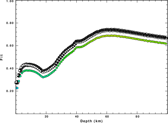
The best fit as a function of depth is given in the following figure:
|
|
Figure 2. Depth sensitivity for waveform mechanism
|
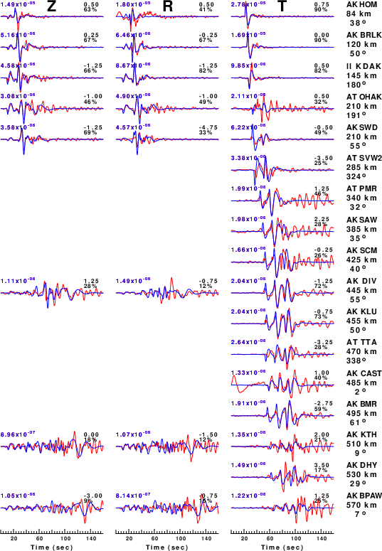
The comparison of the observed and predicted waveforms is given in the next figure. The red traces are the observed and the blue are the predicted.
Each observed-predicted component is plotted to the same scale and peak amplitudes are indicated by the numbers to the left of each trace. A pair of numbers is given in black at the right of each predicted traces. The upper number it the time shift required for maximum correlation between the observed and predicted traces. This time shift is required because the synthetics are not computed at exactly the same distance as the observed, the velocity model used in the predictions may not be perfect and the epicentral parameters may be be off.
A positive time shift indicates that the prediction is too fast and should be delayed to match the observed trace (shift to the right in this figure). A negative value indicates that the prediction is too slow. The lower number gives the percentage of variance reduction to characterize the individual goodness of fit (100% indicates a perfect fit).
The bandpass filter used in the processing and for the display was
hp c 0.02 n 3
lp c 0.10 n 3
|
|
Figure 3. Waveform comparison for selected depth. Red: observed; Blue - predicted. The time shift with respect to the model prediction is indicated. The percent of fit is also indicated. The time scale is relative to the first trace sample.
|
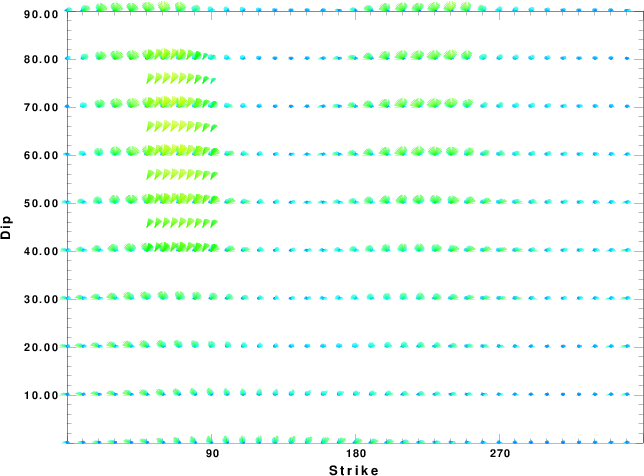
|
|
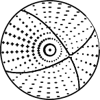
Focal mechanism sensitivity at the preferred depth. The red color indicates a very good fit to the waveforms.
Each solution is plotted as a vector at a given value of strike and dip with the angle of the vector representing the rake angle, measured, with respect to the upward vertical (N) in the figure.
|
A check on the assumed source location is possible by looking at the time shifts between the observed and predicted traces. The time shifts for waveform matching arise for several reasons:
- The origin time and epicentral distance are incorrect
- The velocity model used for the inversion is incorrect
- The velocity model used to define the P-arrival time is not the
same as the velocity model used for the waveform inversion
(assuming that the initial trace alignment is based on the
P arrival time)
Assuming only a mislocation, the time shifts are fit to a functional form:
Time_shift = A + B cos Azimuth + C Sin Azimuth
The time shifts for this inversion lead to the next figure:
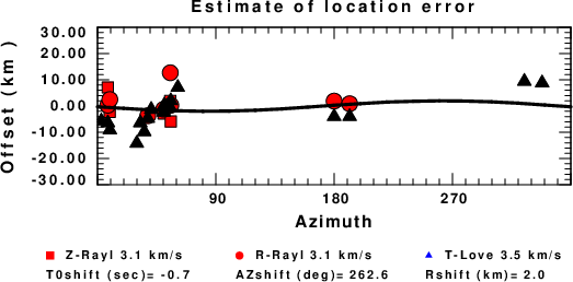
The derived shift in origin time and epicentral coordinates are given at the bottom of the figure.
Velocity Model
The WUS.model used for the waveform synthetic seismograms and for the surface wave eigenfunctions and dispersion is as follows
(The format is in the model96 format of Computer Programs in Seismology).
MODEL.01
Model after     8 iterations
ISOTROPIC
KGS
FLAT EARTH
1-D
CONSTANT VELOCITY
LINE08
LINE09
LINE10
LINE11
      H(KM)   VP(KM/S)   VS(KM/S) RHO(GM/CC)         QP         QS       ETAP       ETAS      FREFP      FREFS
     1.9000     3.4065     2.0089     2.2150  0.302E-02  0.679E-02   0.00       0.00       1.00       1.00
     6.1000     5.5445     3.2953     2.6089  0.349E-02  0.784E-02   0.00       0.00       1.00       1.00
    13.0000     6.2708     3.7396     2.7812  0.212E-02  0.476E-02   0.00       0.00       1.00       1.00
    19.0000     6.4075     3.7680     2.8223  0.111E-02  0.249E-02   0.00       0.00       1.00       1.00
     0.0000     7.9000     4.6200     3.2760  0.164E-10  0.370E-10   0.00       0.00       1.00       1.00
Last Changed Sat Apr 27 01:19:45 PM CDT 2024