The ANSS event ID is usp000j0ct and the event page is at https://earthquake.usgs.gov/earthquakes/eventpage/usp000j0ct/executive.
2011/04/22 00:06:04 63.964 -130.995 5.9 4.1 Yukon, Canada
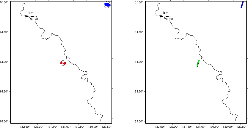
 USGS/SLU Moment Tensor Solution
 ENS  2011/04/22 00:06:04:0  63.96 -130.99   5.9 4.1 Yukon, Canada

 Stations used:
   AK.BAL AK.CCB AK.CTG AK.DHY AK.HDA AK.KLU AK.MCK AK.MDM
   AK.RAG AK.RND AK.SCM AK.TGL AK.WRH AT.MENT AT.SKAG CN.BVCY
   CN.DAWY CN.DLBC CN.HPLN CN.HYT CN.INK CN.SMPN CN.WHY
   CN.YUK1 CN.YUK5 CN.YUK7 IU.COLA US.EGAK US.WRAK

 Filtering commands used:
   hp c 0.02 n 3
   lp c 0.06 n 3

 Best Fitting Double Couple
  Mo = 2.11e+22 dyne-cm
  Mw = 4.15
  Z  = 11 km
  Plane   Strike  Dip  Rake
   NP1       60    90   -10
   NP2      150    80   -180
  Principal Axes:
   Axis    Value   Plunge  Azimuth
    T   2.11e+22      7     105
    N   0.00e+00     80     240
    P  -2.11e+22      7      15

 Moment Tensor: (dyne-cm)
    Component   Value
       Mxx    -1.80e+22
       Mxy    -1.04e+22
       Mxz    -3.18e+21
       Myy     1.80e+22
       Myz     1.84e+21
       Mzz     3.21e+14


                     ---------- P -
                 #-------------   -----
              ####------------------------
             ######------------------------
           ########--------------------------
          ##########--------------------------
         ############---------------------#####
        ##############-----------------#########
        ###############-------------############
       #################---------################
       ##################-----###################
       ##########################################
       ################----##################   #
        ############--------################# T
        #########------------################
         #####----------------#################
          ----------------------##############
           ----------------------############
             ---------------------#########
              ----------------------######
                 ---------------------#
                     --------------


 Global CMT Convention Moment Tensor:
      R          T          P
  3.21e+14  -3.18e+21  -1.84e+21
 -3.18e+21  -1.80e+22   1.04e+22
 -1.84e+21   1.04e+22   1.80e+22


Details of the solution is found at

http://www.eas.slu.edu/eqc/eqc_mt/MECH.NA/20110422000604/index.html
|
      STK = 60
      DIP = 90
     RAKE = -10
       MW = 4.15
       HS = 11.0
The NDK file is 20110422000604.ndk The waveform inversion is preferred.
Given the availability of digital waveforms for determination of the moment tensor, this section documents the added processing leading to mLg, if appropriate to the region, and ML by application of the respective IASPEI formulae. As a research study, the linear distance term of the IASPEI formula for ML is adjusted to remove a linear distance trend in residuals to give a regionally defined ML. The defined ML uses horizontal component recordings, but the same procedure is applied to the vertical components since there may be some interest in vertical component ground motions. Residual plots versus distance may indicate interesting features of ground motion scaling in some distance ranges. A residual plot of the regionalized magnitude is given as a function of distance and azimuth, since data sets may transcend different wave propagation provinces.
|
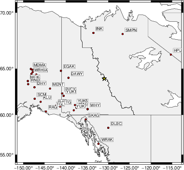
The focal mechanism was determined using broadband seismic waveforms. The location of the event (star) and the stations used for (red) the waveform inversion are shown in the next figure.
|
|
|
The program wvfgrd96 was used with good traces observed at short distance to determine the focal mechanism, depth and seismic moment. This technique requires a high quality signal and well determined velocity model for the Green's functions. To the extent that these are the quality data, this type of mechanism should be preferred over the radiation pattern technique which requires the separate step of defining the pressure and tension quadrants and the correct strike.
The observed and predicted traces are filtered using the following gsac commands:
hp c 0.02 n 3
lp c 0.06 n 3
The results of this grid search are as follow:
           DEPTH  STK   DIP  RAKE   MW    FIT
WVFGRD96    0.5    65    90   -15   3.96 0.4235
WVFGRD96    1.0    65    90   -15   3.98 0.4505
WVFGRD96    2.0    65    90     0   4.01 0.4994
WVFGRD96    3.0    65    90     0   4.04 0.5353
WVFGRD96    4.0   240    85    -5   4.07 0.5625
WVFGRD96    5.0   240    85    -5   4.09 0.5813
WVFGRD96    6.0   240    80    -5   4.10 0.5952
WVFGRD96    7.0   240    80    -5   4.11 0.6054
WVFGRD96    8.0   240    90    10   4.13 0.6132
WVFGRD96    9.0   240    90    10   4.14 0.6200
WVFGRD96   10.0    60    85   -10   4.15 0.6259
WVFGRD96   11.0    60    90   -10   4.15 0.6277
WVFGRD96   12.0   240    90    10   4.16 0.6274
WVFGRD96   13.0   240    90    10   4.17 0.6251
WVFGRD96   14.0    60    90    -5   4.17 0.6218
WVFGRD96   15.0   240    90     5   4.18 0.6175
WVFGRD96   16.0    60    90    -5   4.18 0.6136
WVFGRD96   17.0   240    90     5   4.19 0.6088
WVFGRD96   18.0    60    85     0   4.20 0.6033
WVFGRD96   19.0   240    90     0   4.21 0.5979
WVFGRD96   20.0    60    85     0   4.21 0.5941
WVFGRD96   21.0   240    90    -5   4.22 0.5864
WVFGRD96   22.0   240    90    -5   4.23 0.5789
WVFGRD96   23.0    60    85     0   4.23 0.5709
WVFGRD96   24.0    60    85     0   4.24 0.5621
WVFGRD96   25.0    60    85     0   4.24 0.5530
WVFGRD96   26.0    60    85     0   4.25 0.5432
WVFGRD96   27.0    60    85     0   4.25 0.5336
WVFGRD96   28.0    60    85     0   4.26 0.5239
WVFGRD96   29.0   240    90    -5   4.27 0.5135
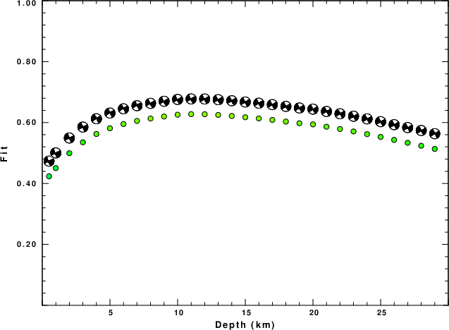
The best solution is
WVFGRD96 11.0 60 90 -10 4.15 0.6277
The mechanism corresponding to the best fit is
|
|
|
The best fit as a function of depth is given in the following figure:
|
|
|
The comparison of the observed and predicted waveforms is given in the next figure. The red traces are the observed and the blue are the predicted. Each observed-predicted component is plotted to the same scale and peak amplitudes are indicated by the numbers to the left of each trace. A pair of numbers is given in black at the right of each predicted traces. The upper number it the time shift required for maximum correlation between the observed and predicted traces. This time shift is required because the synthetics are not computed at exactly the same distance as the observed, the velocity model used in the predictions may not be perfect and the epicentral parameters may be be off. A positive time shift indicates that the prediction is too fast and should be delayed to match the observed trace (shift to the right in this figure). A negative value indicates that the prediction is too slow. The lower number gives the percentage of variance reduction to characterize the individual goodness of fit (100% indicates a perfect fit).
The bandpass filter used in the processing and for the display was
hp c 0.02 n 3
lp c 0.06 n 3
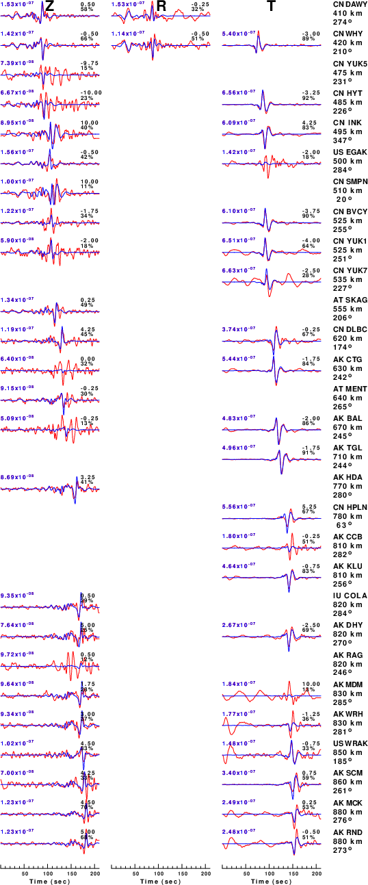
|
| Figure 3. Waveform comparison for selected depth. Red: observed; Blue - predicted. The time shift with respect to the model prediction is indicated. The percent of fit is also indicated. The time scale is relative to the first trace sample. |
|
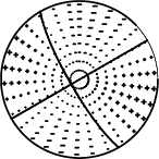
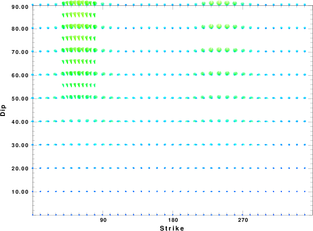
| Focal mechanism sensitivity at the preferred depth. The red color indicates a very good fit to the waveforms. Each solution is plotted as a vector at a given value of strike and dip with the angle of the vector representing the rake angle, measured, with respect to the upward vertical (N) in the figure. |
A check on the assumed source location is possible by looking at the time shifts between the observed and predicted traces. The time shifts for waveform matching arise for several reasons:
Time_shift = A + B cos Azimuth + C Sin Azimuth
The time shifts for this inversion lead to the next figure:
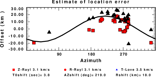
The derived shift in origin time and epicentral coordinates are given at the bottom of the figure.
The CUS.model used for the waveform synthetic seismograms and for the surface wave eigenfunctions and dispersion is as follows (The format is in the model96 format of Computer Programs in Seismology).
MODEL.01
CUS Model with Q from simple gamma values
ISOTROPIC
KGS
FLAT EARTH
1-D
CONSTANT VELOCITY
LINE08
LINE09
LINE10
LINE11
  H(KM) VP(KM/S) VS(KM/S) RHO(GM/CC)   QP   QS  ETAP  ETAS  FREFP  FREFS
  1.0000  5.0000  2.8900  2.5000 0.172E-02 0.387E-02 0.00  0.00  1.00  1.00
  9.0000  6.1000  3.5200  2.7300 0.160E-02 0.363E-02 0.00  0.00  1.00  1.00
 10.0000  6.4000  3.7000  2.8200 0.149E-02 0.336E-02 0.00  0.00  1.00  1.00
 20.0000  6.7000  3.8700  2.9020 0.000E-04 0.000E-04 0.00  0.00  1.00  1.00
  0.0000  8.1500  4.7000  3.3640 0.194E-02 0.431E-02 0.00  0.00  1.00  1.00