Location
Location ANSS
The ANSS event ID is ak0113v5ldih and the event page is at
https://earthquake.usgs.gov/earthquakes/eventpage/ak0113v5ldih/executive.
2011/03/25 14:19:38 62.659 -151.482 118.5 4.4 Alaska
Focal Mechanism
USGS/SLU Moment Tensor Solution
ENS 2011/03/25 14:19:38:0 62.66 -151.48 118.5 4.4 Alaska
Stations used:
AK.BPAW AK.CAST AK.DHY AK.KTH AK.MCK AK.MDM AK.MLY AK.PPLA
AK.RC01 AK.RND AK.SAW AK.SCM AK.SWD AK.TRF AK.WRH AT.PMR
Filtering commands used:
hp c 0.02 n 3
lp c 0.08 n 3
Best Fitting Double Couple
Mo = 4.22e+22 dyne-cm
Mw = 4.35
Z = 108 km
Plane Strike Dip Rake
NP1 80 80 -50
NP2 182 41 -165
Principal Axes:
Axis Value Plunge Azimuth
T 4.22e+22 24 140
N 0.00e+00 39 252
P -4.22e+22 41 27
Moment Tensor: (dyne-cm)
Component Value
Mxx 1.59e+21
Mxy -2.70e+22
Mxz -3.07e+22
Myy 9.46e+21
Myz 6.36e+20
Mzz -1.10e+22
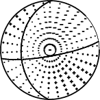
#####---------
######----------------
########--------------------
#######-----------------------
########------------- ----------
########-------------- P -----------
########--------------- ------------
#########-------------------------------
########--------------------------------
#########-------------------------------##
#########--------------------------#######
#########--------------------#############
#########-----------######################
--------################################
---------###############################
--------##############################
--------################### ######
--------################## T #####
-------################# ###
-------#####################
------################
----##########
Global CMT Convention Moment Tensor:
R T P
-1.10e+22 -3.07e+22 -6.36e+20
-3.07e+22 1.59e+21 2.70e+22
-6.36e+20 2.70e+22 9.46e+21
Details of the solution is found at
http://www.eas.slu.edu/eqc/eqc_mt/MECH.NA/20110325141938/index.html
|
Preferred Solution
The preferred solution from an analysis of the surface-wave spectral amplitude radiation pattern, waveform inversion or first motion observations is
      STK = 80
      DIP = 80
     RAKE = -50
       MW = 4.35
       HS = 108.0
The NDK file is 20110325141938.ndk
The waveform inversion is preferred.
Magnitudes
Given the availability of digital waveforms for determination of the moment tensor, this section documents the added processing leading to mLg, if appropriate to the region, and ML by application of the respective IASPEI formulae. As a research study, the linear distance term of the IASPEI formula
for ML is adjusted to remove a linear distance trend in residuals to give a regionally defined ML. The defined ML uses horizontal component recordings, but the same procedure is applied to the vertical components since there may be some interest in vertical component ground motions. Residual plots versus distance may indicate interesting features of ground motion scaling in some distance ranges. A residual plot of the regionalized magnitude is given as a function of distance and azimuth, since data sets may transcend different wave propagation provinces.
ML Magnitude
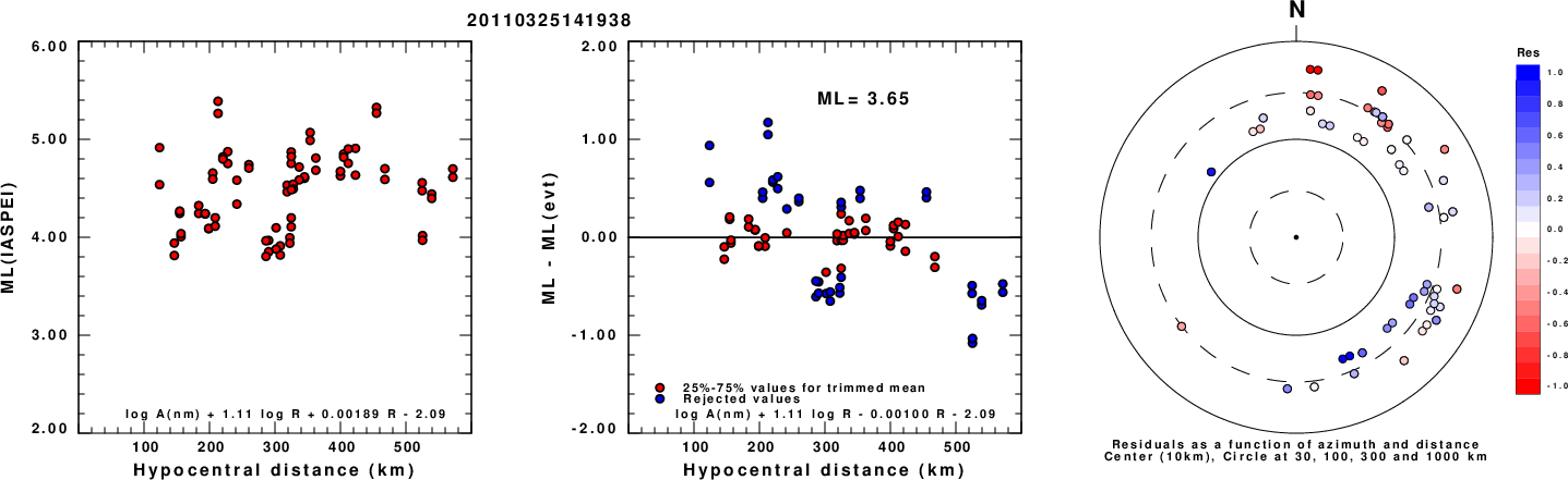
Left: ML computed using the IASPEI formula for Horizontal components. Center: ML residuals computed using a modified IASPEI formula that accounts for path specific attenuation; the values used for the trimmed mean are indicated. The ML relation used for each figure is given at the bottom of each plot.
Right: Residuals from new relation as a function of distance and azimuth.
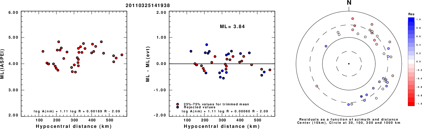
Left: ML computed using the IASPEI formula for Vertical components (research). Center: ML residuals computed using a modified IASPEI formula that accounts for path specific attenuation; the values used for the trimmed mean are indicated. The ML relation used for each figure is given at the bottom of each plot.
Right: Residuals from new relation as a function of distance and azimuth.
Context
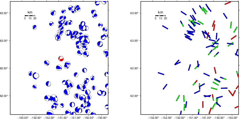
The left panel of the next figure presents the focal mechanism for this earthquake (red) in the context of other nearby events (blue) in the SLU Moment Tensor Catalog. The right panel shows the inferred direction of maximum compressive stress and the type of faulting (green is strike-slip, red is normal, blue is thrust; oblique is shown by a combination of colors). Thus context plot is useful for assessing the appropriateness of the moment tensor of this event.
Waveform Inversion using wvfgrd96
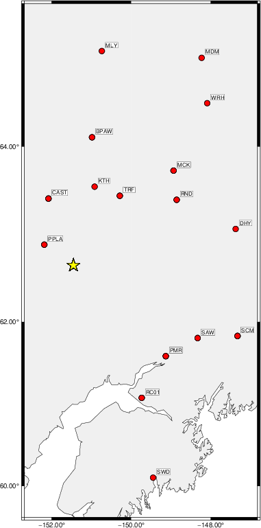
The focal mechanism was determined using broadband seismic waveforms. The location of the event (star) and the
stations used for (red) the waveform inversion are shown in the next figure.
|
|
Location of broadband stations used for waveform inversion
|
The program wvfgrd96 was used with good traces observed at short distance to determine the focal mechanism, depth and seismic moment. This technique requires a high quality signal and well determined velocity model for the Green's functions. To the extent that these are the quality data, this type of mechanism should be preferred over the radiation pattern technique which requires the separate step of defining the pressure and tension quadrants and the correct strike.
The observed and predicted traces are filtered using the following gsac commands:
hp c 0.02 n 3
lp c 0.08 n 3
The results of this grid search are as follow:
           DEPTH  STK   DIP  RAKE   MW    FIT
WVFGRD96    2.0   195    70    20   3.42 0.2492
WVFGRD96    4.0    10    70   -10   3.50 0.2576
WVFGRD96    6.0   315    60    20   3.57 0.2760
WVFGRD96    8.0   315    60    20   3.64 0.2960
WVFGRD96   10.0   315    60    20   3.67 0.3067
WVFGRD96   12.0   135    65    25   3.71 0.3139
WVFGRD96   14.0   130    65    20   3.73 0.3228
WVFGRD96   16.0   130    65    20   3.76 0.3291
WVFGRD96   18.0   105    65     5   3.78 0.3366
WVFGRD96   20.0   105    65     5   3.80 0.3483
WVFGRD96   22.0   105    65     5   3.82 0.3589
WVFGRD96   24.0   105    70     5   3.84 0.3696
WVFGRD96   26.0   105    65     5   3.86 0.3796
WVFGRD96   28.0   105    65     5   3.88 0.3877
WVFGRD96   30.0   110    60    15   3.91 0.3941
WVFGRD96   32.0   110    65    15   3.92 0.4007
WVFGRD96   34.0   110    65    15   3.94 0.4065
WVFGRD96   36.0   100    80   -20   3.94 0.4119
WVFGRD96   38.0   100    80   -20   3.97 0.4188
WVFGRD96   40.0    95    75   -30   4.04 0.4262
WVFGRD96   42.0    95    70   -30   4.06 0.4287
WVFGRD96   44.0    95    70   -25   4.08 0.4287
WVFGRD96   46.0    95    70   -25   4.09 0.4287
WVFGRD96   48.0    95    60   -20   4.12 0.4320
WVFGRD96   50.0    95    60   -15   4.14 0.4347
WVFGRD96   52.0    95    60   -20   4.15 0.4385
WVFGRD96   54.0    95    60   -20   4.16 0.4420
WVFGRD96   56.0    95    60   -15   4.18 0.4474
WVFGRD96   58.0    95    65   -20   4.18 0.4525
WVFGRD96   60.0    95    60   -15   4.21 0.4592
WVFGRD96   62.0    95    60   -15   4.22 0.4645
WVFGRD96   64.0    90    75   -35   4.20 0.4705
WVFGRD96   66.0    90    75   -35   4.21 0.4792
WVFGRD96   68.0    90    75   -40   4.22 0.4880
WVFGRD96   70.0    85    75   -45   4.23 0.4956
WVFGRD96   72.0    85    75   -45   4.24 0.5055
WVFGRD96   74.0    85    75   -45   4.25 0.5152
WVFGRD96   76.0    85    70   -40   4.26 0.5234
WVFGRD96   78.0    85    70   -40   4.27 0.5328
WVFGRD96   80.0    85    75   -45   4.27 0.5408
WVFGRD96   82.0    85    75   -40   4.28 0.5493
WVFGRD96   84.0    85    75   -40   4.29 0.5582
WVFGRD96   86.0    85    75   -40   4.30 0.5643
WVFGRD96   88.0    80    75   -45   4.31 0.5725
WVFGRD96   90.0    80    75   -45   4.32 0.5782
WVFGRD96   92.0    80    75   -45   4.32 0.5845
WVFGRD96   94.0    80    75   -45   4.33 0.5878
WVFGRD96   96.0    80    75   -45   4.33 0.5913
WVFGRD96   98.0    80    80   -50   4.33 0.5936
WVFGRD96  100.0    80    80   -50   4.34 0.5975
WVFGRD96  101.0    80    80   -50   4.34 0.5982
WVFGRD96  102.0    80    80   -50   4.34 0.5983
WVFGRD96  103.0    80    80   -50   4.34 0.6006
WVFGRD96  104.0    80    80   -50   4.34 0.6006
WVFGRD96  105.0    80    80   -50   4.35 0.6007
WVFGRD96  106.0    80    80   -50   4.35 0.6002
WVFGRD96  107.0    80    80   -50   4.35 0.6008
WVFGRD96  108.0    80    80   -50   4.35 0.6009
WVFGRD96  109.0    80    80   -45   4.35 0.6007
WVFGRD96  110.0    80    80   -45   4.36 0.6000
WVFGRD96  111.0    80    80   -45   4.36 0.5994
WVFGRD96  112.0    80    80   -45   4.36 0.5997
WVFGRD96  113.0    85    85   -45   4.35 0.5992
WVFGRD96  114.0    85    85   -45   4.35 0.5989
WVFGRD96  115.0    85    85   -45   4.35 0.5978
WVFGRD96  116.0    85    85   -45   4.36 0.5977
WVFGRD96  117.0    85    85   -45   4.36 0.5982
WVFGRD96  118.0    85    85   -45   4.36 0.5968
WVFGRD96  119.0    85    85   -45   4.36 0.5961
WVFGRD96  120.0    85    85   -45   4.36 0.5943
WVFGRD96  121.0    85    85   -45   4.36 0.5941
WVFGRD96  122.0    85    85   -45   4.36 0.5937
WVFGRD96  123.0    85    85   -45   4.36 0.5916
WVFGRD96  124.0    85    85   -45   4.37 0.5905
WVFGRD96  125.0    85    85   -45   4.37 0.5885
The best solution is
WVFGRD96 108.0 80 80 -50 4.35 0.6009
The mechanism corresponding to the best fit is
|
|
Figure 1. Waveform inversion focal mechanism
|
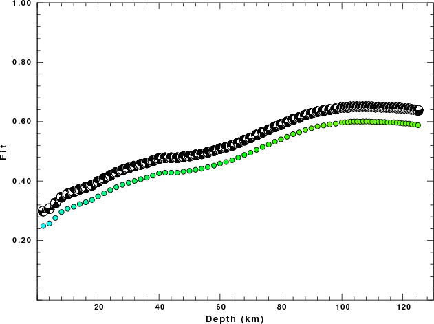
The best fit as a function of depth is given in the following figure:
|
|
Figure 2. Depth sensitivity for waveform mechanism
|
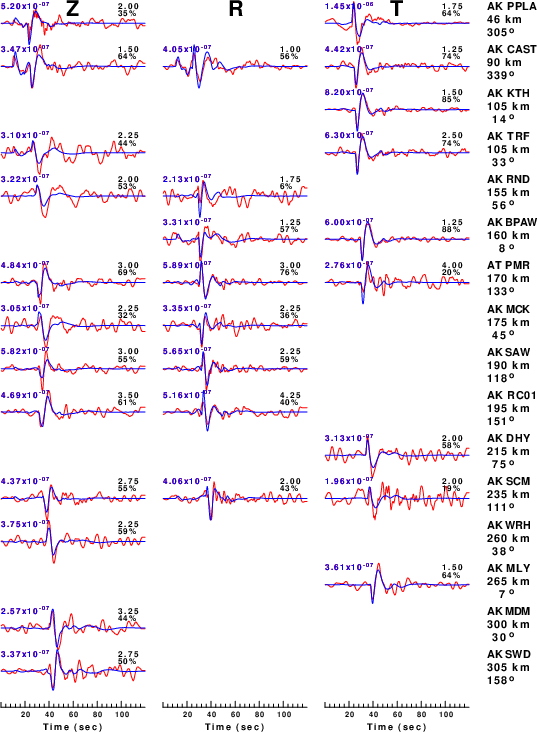
The comparison of the observed and predicted waveforms is given in the next figure. The red traces are the observed and the blue are the predicted.
Each observed-predicted component is plotted to the same scale and peak amplitudes are indicated by the numbers to the left of each trace. A pair of numbers is given in black at the right of each predicted traces. The upper number it the time shift required for maximum correlation between the observed and predicted traces. This time shift is required because the synthetics are not computed at exactly the same distance as the observed, the velocity model used in the predictions may not be perfect and the epicentral parameters may be be off.
A positive time shift indicates that the prediction is too fast and should be delayed to match the observed trace (shift to the right in this figure). A negative value indicates that the prediction is too slow. The lower number gives the percentage of variance reduction to characterize the individual goodness of fit (100% indicates a perfect fit).
The bandpass filter used in the processing and for the display was
hp c 0.02 n 3
lp c 0.08 n 3
|
|
Figure 3. Waveform comparison for selected depth. Red: observed; Blue - predicted. The time shift with respect to the model prediction is indicated. The percent of fit is also indicated. The time scale is relative to the first trace sample.
|
|
|
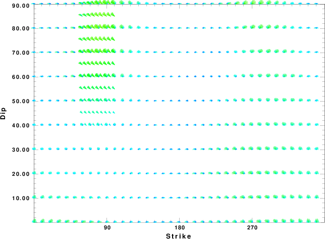
Focal mechanism sensitivity at the preferred depth. The red color indicates a very good fit to the waveforms.
Each solution is plotted as a vector at a given value of strike and dip with the angle of the vector representing the rake angle, measured, with respect to the upward vertical (N) in the figure.
|
A check on the assumed source location is possible by looking at the time shifts between the observed and predicted traces. The time shifts for waveform matching arise for several reasons:
- The origin time and epicentral distance are incorrect
- The velocity model used for the inversion is incorrect
- The velocity model used to define the P-arrival time is not the
same as the velocity model used for the waveform inversion
(assuming that the initial trace alignment is based on the
P arrival time)
Assuming only a mislocation, the time shifts are fit to a functional form:
Time_shift = A + B cos Azimuth + C Sin Azimuth
The time shifts for this inversion lead to the next figure:
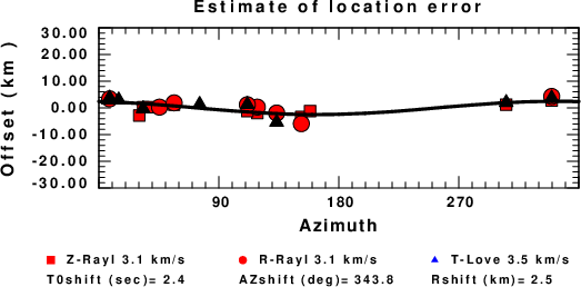
The derived shift in origin time and epicentral coordinates are given at the bottom of the figure.
Velocity Model
The WUS.model used for the waveform synthetic seismograms and for the surface wave eigenfunctions and dispersion is as follows
(The format is in the model96 format of Computer Programs in Seismology).
MODEL.01
Model after     8 iterations
ISOTROPIC
KGS
FLAT EARTH
1-D
CONSTANT VELOCITY
LINE08
LINE09
LINE10
LINE11
      H(KM)   VP(KM/S)   VS(KM/S) RHO(GM/CC)         QP         QS       ETAP       ETAS      FREFP      FREFS
     1.9000     3.4065     2.0089     2.2150  0.302E-02  0.679E-02   0.00       0.00       1.00       1.00
     6.1000     5.5445     3.2953     2.6089  0.349E-02  0.784E-02   0.00       0.00       1.00       1.00
    13.0000     6.2708     3.7396     2.7812  0.212E-02  0.476E-02   0.00       0.00       1.00       1.00
    19.0000     6.4075     3.7680     2.8223  0.111E-02  0.249E-02   0.00       0.00       1.00       1.00
     0.0000     7.9000     4.6200     3.2760  0.164E-10  0.370E-10   0.00       0.00       1.00       1.00
Last Changed Sat Apr 27 12:29:15 PM CDT 2024