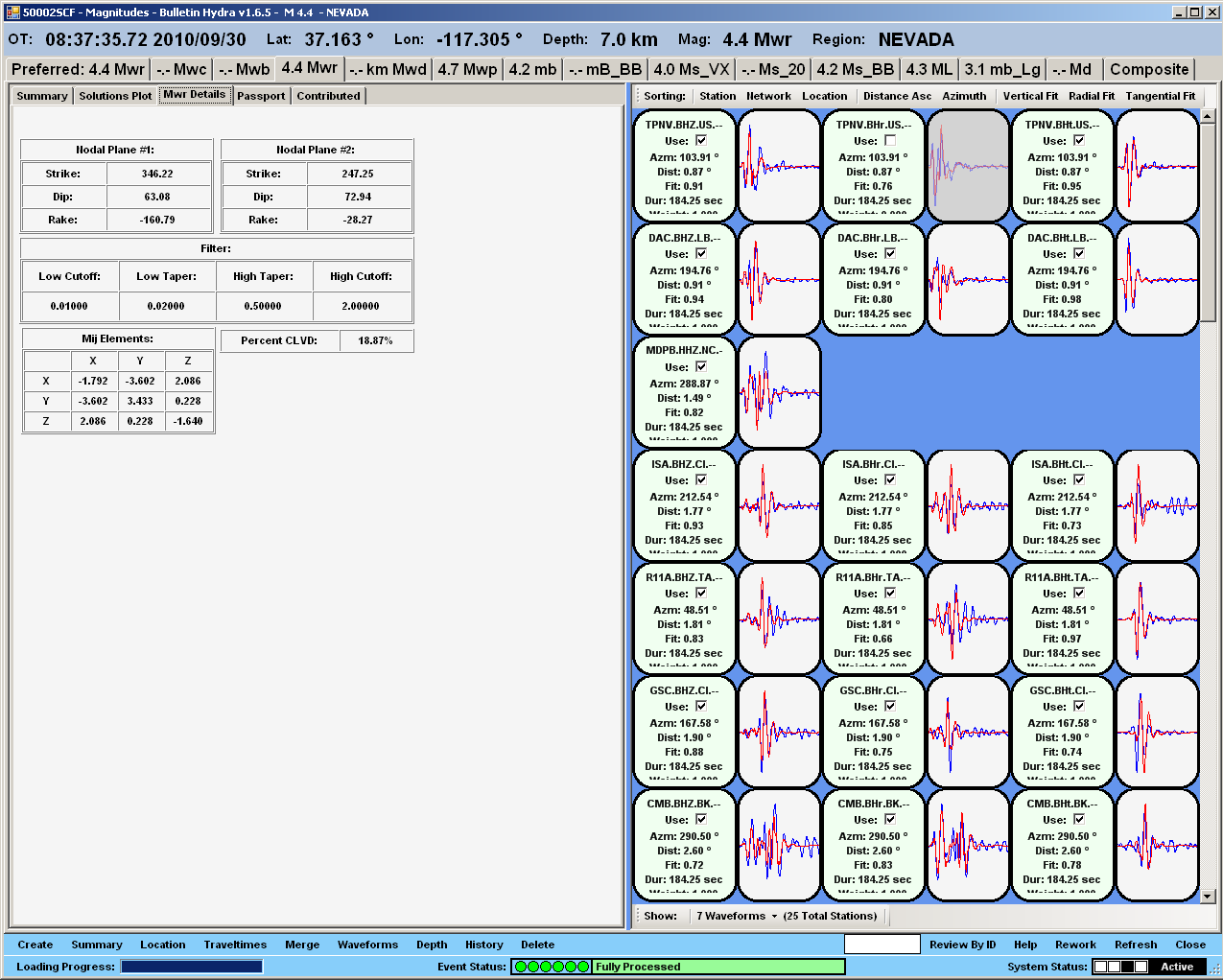
Location
Location ANSS
The ANSS event ID is nn00429638 and the event page is at
https://earthquake.usgs.gov/earthquakes/eventpage/nn00429638/executive.
2010/09/30 08:37:36 37.140 -117.380 6.5 4.3 Nevada
Focal Mechanism
 USGS/SLU Moment Tensor Solution
 ENS  2010/09/30 08:37:36:0  37.14 -117.38   6.5 4.3 Nevada

 Stations used:
   BK.CMB BK.MOD CI.BAR CI.GLA CI.GSC CI.ISA CI.LDF CI.MWC
   CI.PASC II.PFO LB.BMN LB.DAC NC.MDPB US.DUG US.ELK US.TPNV
   US.WUAZ US.WVOR UU.CCUT UU.CVRU UU.LCMT UU.MPU UU.MTPU
   UU.NLU UU.PKCU UU.PSUT UU.SZCU UU.TCRU UU.TMU

 Filtering commands used:
   hp c 0.02 n 3
   lp c 0.06 n 3

 Best Fitting Double Couple
  Mo = 4.84e+22 dyne-cm
  Mw = 4.39
  Z  = 12 km
  Plane   Strike  Dip  Rake
   NP1      250    75   -20
   NP2      345    71   -164
  Principal Axes:
   Axis    Value   Plunge  Azimuth
    T   4.84e+22      3     298
    N   0.00e+00     65      35
    P  -4.84e+22     25     207

 Moment Tensor: (dyne-cm)
    Component   Value
       Mxx    -2.09e+22
       Mxy    -3.63e+22
       Mxz     1.75e+22
       Myy     2.92e+22
       Myz     6.16e+21
       Mzz    -8.28e+21


                     ##------------
                 ########--------------
              #############---------------
             ###############---------------
            #################----------------
          T ##################----------------
            ##################-----------------
        #######################------###########
        ######################--################
       ##################-------#################
       #############-------------################
       ##########----------------################
       #######--------------------###############
        ###-----------------------##############
        #-------------------------##############
         -------------------------#############
          -------------------------###########
           --------   -------------##########
             ------ P ------------#########
              -----   ------------########
                 -----------------#####
                     ------------##


 Global CMT Convention Moment Tensor:
      R          T          P
 -8.28e+21   1.75e+22  -6.16e+21
  1.75e+22  -2.09e+22   3.63e+22
 -6.16e+21   3.63e+22   2.92e+22


Details of the solution is found at

http://www.eas.slu.edu/eqc/eqc_mt/MECH.NA/20100930083736/index.html
|
Preferred Solution
The preferred solution from an analysis of the surface-wave spectral amplitude radiation pattern, waveform inversion or first motion observations is
      STK = 250
      DIP = 75
     RAKE = -20
       MW = 4.39
       HS = 12.0
The NDK file is 20100930083736.ndk
The waveform inversion is preferred.
Moment Tensor Comparison
The following compares this source inversion to those provided by others. The purpose is to look for major differences and also to note slight differences that might be inherent to the processing procedure. For completeness the USGS/SLU solution is repeated from above.
| SLU |
USGSMT |
UNR |
 USGS/SLU Moment Tensor Solution
 ENS  2010/09/30 08:37:36:0  37.14 -117.38   6.5 4.3 Nevada

 Stations used:
   BK.CMB BK.MOD CI.BAR CI.GLA CI.GSC CI.ISA CI.LDF CI.MWC
   CI.PASC II.PFO LB.BMN LB.DAC NC.MDPB US.DUG US.ELK US.TPNV
   US.WUAZ US.WVOR UU.CCUT UU.CVRU UU.LCMT UU.MPU UU.MTPU
   UU.NLU UU.PKCU UU.PSUT UU.SZCU UU.TCRU UU.TMU

 Filtering commands used:
   hp c 0.02 n 3
   lp c 0.06 n 3

 Best Fitting Double Couple
  Mo = 4.84e+22 dyne-cm
  Mw = 4.39
  Z  = 12 km
  Plane   Strike  Dip  Rake
   NP1      250    75   -20
   NP2      345    71   -164
  Principal Axes:
   Axis    Value   Plunge  Azimuth
    T   4.84e+22      3     298
    N   0.00e+00     65      35
    P  -4.84e+22     25     207

 Moment Tensor: (dyne-cm)
    Component   Value
       Mxx    -2.09e+22
       Mxy    -3.63e+22
       Mxz     1.75e+22
       Myy     2.92e+22
       Myz     6.16e+21
       Mzz    -8.28e+21


                     ##------------
                 ########--------------
              #############---------------
             ###############---------------
            #################----------------
          T ##################----------------
            ##################-----------------
        #######################------###########
        ######################--################
       ##################-------#################
       #############-------------################
       ##########----------------################
       #######--------------------###############
        ###-----------------------##############
        #-------------------------##############
         -------------------------#############
          -------------------------###########
           --------   -------------##########
             ------ P ------------#########
              -----   ------------########
                 -----------------#####
                     ------------##


 Global CMT Convention Moment Tensor:
      R          T          P
 -8.28e+21   1.75e+22  -6.16e+21
  1.75e+22  -2.09e+22   3.63e+22
 -6.16e+21   3.63e+22   2.92e+22


Details of the solution is found at

http://www.eas.slu.edu/eqc/eqc_mt/MECH.NA/20100930083736/index.html
|
|
|
|
|
REVIEWED BY NSL STAFF

Event ID:317359
Origin ID:755037
Seismic Moment Tensor Solution

2010/09/30 (273) 08:37:35.00 37.1385 -117.3803 755037
	Depth =  14.0 (km)
	Mw    =  4.34
	Mo    =  3.98x10^22 (dyne x cm)

	Percent Double Couple =  98 %
	Percent CLVD          =   2 %
	no ISO calculated
	Epsilon=-0.01
	 Percent Variance Reduction =  52.72 %
	 Total Fit                  =  15.42
	Major Double Couple
		            strike dip   rake
		Nodal Plane 1: 342  82  179
		Nodal Plane 2:  72  89    8

	DEVIATORIC MOMENT TENSOR

	Moment Tensor Elements: Spherical Coordinates
		Mrr= -0.04 Mtt= -2.29 Mff=  2.32
		Mrt=  0.48 Mrf=  0.21 Mtf=  3.20 EXP=22


	Moment Tensor Elements: Cartesian Coordinates
		-2.29 -3.20  0.48
		-3.20  2.32 -0.21
		 0.48 -0.21 -0.04

	Eigenvalues:
		T-axis eigenvalue=  4.00
		N-axis eigenvalue= -0.05
		P-axis eigenvalue= -3.95

	Eigenvalues and eigenvectors of the Major Double Couple:
		T-axis ev= 4.00 trend=297 plunge=6
		N-axis ev= 0.00 trend=77 plunge=82
		P-axis ev=-4.00 trend=207 plunge=5

	Maximum Azmuithal Gap=115 Distance to Nearest Station= 75.9 (km)

	Number of Stations (D=Displacement/V=Velocity) Used=5 (defining only)

	 TIN.CI.D FUR.CI.D DAC.LB.D MLAC.CI.D
	 R11A.TA.D


              ###--------------
          ########-----------------
        ###########------------------
      #############--------------------
     ###############--------------------
    #################--------------------
 T ###################---------------------
   ####################--------------------
 ######################-----------------####
 #######################----------##########
 ########################---#################
 ############################################
 ############################################
 #################-------####################
 ###########-------------###################
 #####--------------------##################
  ------------------------#################
   ------------------------################
   ------------------------###############
     -----------------------#############
      ----------------------###########
        -   ----------------#########
          P -----------------######
              ---------------###


All Stations defining and nondefining:
Station.Net 	Def 	Distance 	Azi    	Bazi  	lo-f 	hi-f vmodel
            	    	(km)     	(deg)  	(deg) 	(Hz) 	(Hz)
TIN.CI (D) 	Y 	    75.9  	263  	 82  	0.020 	0.080 TIN.CI.wus.glib
FUR.CI (D) 	Y 	    87.5  	148  	328  	0.020 	0.080 FUR.CI.wus.glib
DAC.LB (D) 	Y 	    97.2  	191  	 11  	0.020 	0.080 DAC.LB.wus.glib
MLAC.CI (D) 	Y 	   140.0  	293  	113  	0.020 	0.080 MLAC.CI.wus.glib
R11A.TA (D) 	Y 	   207.0  	 49  	230  	0.020 	0.080 R11A.TA.wus.glib

 (V)-velocity (D)-Displacement

Author: www-data
Date: 2010/09/30 16:51:36

mtinv Version 2.1_DEVEL OCT2008
|

http://www.seismo.unr.edu/Events/main.php?evid=317359
|
Magnitudes
Given the availability of digital waveforms for determination of the moment tensor, this section documents the added processing leading to mLg, if appropriate to the region, and ML by application of the respective IASPEI formulae. As a research study, the linear distance term of the IASPEI formula
for ML is adjusted to remove a linear distance trend in residuals to give a regionally defined ML. The defined ML uses horizontal component recordings, but the same procedure is applied to the vertical components since there may be some interest in vertical component ground motions. Residual plots versus distance may indicate interesting features of ground motion scaling in some distance ranges. A residual plot of the regionalized magnitude is given as a function of distance and azimuth, since data sets may transcend different wave propagation provinces.
ML Magnitude
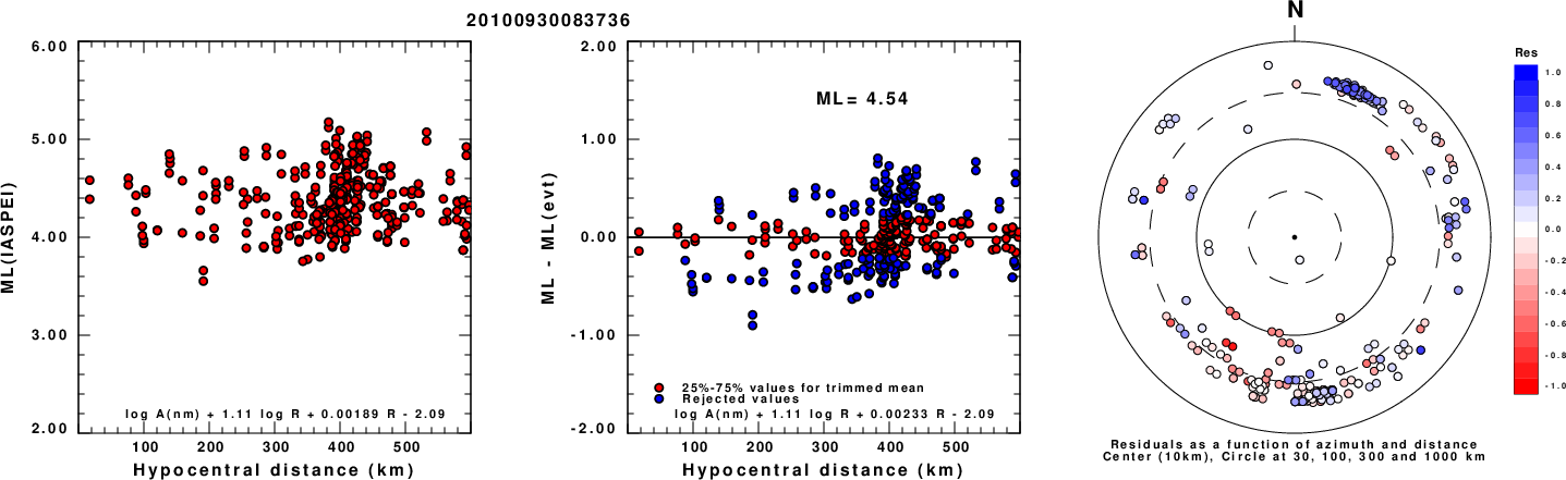
Left: ML computed using the IASPEI formula for Horizontal components. Center: ML residuals computed using a modified IASPEI formula that accounts for path specific attenuation; the values used for the trimmed mean are indicated. The ML relation used for each figure is given at the bottom of each plot.
Right: Residuals from new relation as a function of distance and azimuth.
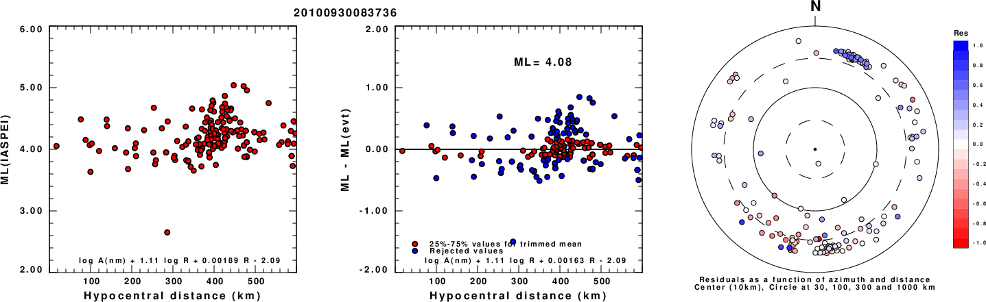
Left: ML computed using the IASPEI formula for Vertical components (research). Center: ML residuals computed using a modified IASPEI formula that accounts for path specific attenuation; the values used for the trimmed mean are indicated. The ML relation used for each figure is given at the bottom of each plot.
Right: Residuals from new relation as a function of distance and azimuth.
Context
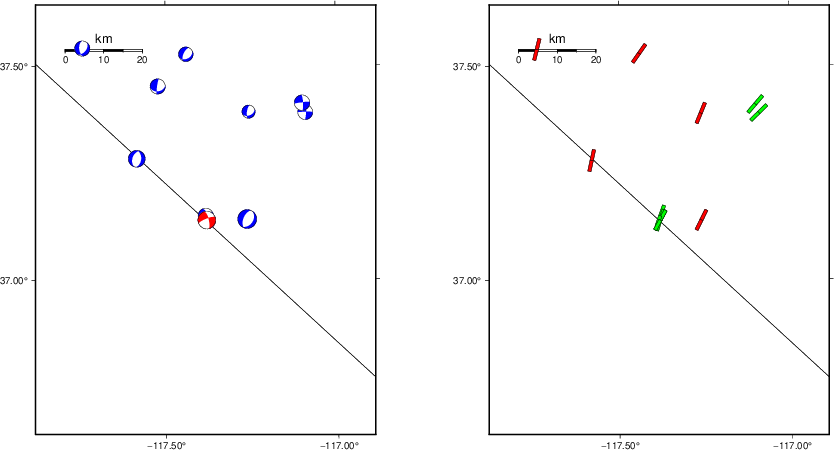
The left panel of the next figure presents the focal mechanism for this earthquake (red) in the context of other nearby events (blue) in the SLU Moment Tensor Catalog. The right panel shows the inferred direction of maximum compressive stress and the type of faulting (green is strike-slip, red is normal, blue is thrust; oblique is shown by a combination of colors). Thus context plot is useful for assessing the appropriateness of the moment tensor of this event.
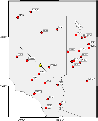
Waveform Inversion using wvfgrd96
The focal mechanism was determined using broadband seismic waveforms. The location of the event (star) and the
stations used for (red) the waveform inversion are shown in the next figure.
|
|
Location of broadband stations used for waveform inversion
|
The program wvfgrd96 was used with good traces observed at short distance to determine the focal mechanism, depth and seismic moment. This technique requires a high quality signal and well determined velocity model for the Green's functions. To the extent that these are the quality data, this type of mechanism should be preferred over the radiation pattern technique which requires the separate step of defining the pressure and tension quadrants and the correct strike.
The observed and predicted traces are filtered using the following gsac commands:
hp c 0.02 n 3
lp c 0.06 n 3
The results of this grid search are as follow:
           DEPTH  STK   DIP  RAKE   MW    FIT
WVFGRD96    0.5    75    75    10   3.96 0.3007
WVFGRD96    1.0   255    80    10   3.99 0.3258
WVFGRD96    2.0   255    80    15   4.09 0.4019
WVFGRD96    3.0    80    55    20   4.19 0.4477
WVFGRD96    4.0    80    55    15   4.21 0.4851
WVFGRD96    5.0    75    60     5   4.23 0.5173
WVFGRD96    6.0    70    65   -10   4.26 0.5513
WVFGRD96    7.0   245    65   -30   4.30 0.5864
WVFGRD96    8.0   245    65   -35   4.34 0.6338
WVFGRD96    9.0   245    65   -30   4.36 0.6651
WVFGRD96   10.0   245    65   -30   4.37 0.6832
WVFGRD96   11.0   245    70   -25   4.39 0.6925
WVFGRD96   12.0   250    75   -20   4.39 0.6982
WVFGRD96   13.0   250    75   -20   4.40 0.6979
WVFGRD96   14.0   250    80   -20   4.41 0.6923
WVFGRD96   15.0   250    80   -20   4.41 0.6832
WVFGRD96   16.0   250    80   -15   4.42 0.6716
WVFGRD96   17.0   250    80   -15   4.43 0.6571
WVFGRD96   18.0   250    80   -15   4.43 0.6418
WVFGRD96   19.0   250    80   -15   4.43 0.6244
WVFGRD96   20.0   250    80   -15   4.44 0.6067
WVFGRD96   21.0   250    80   -15   4.44 0.5888
WVFGRD96   22.0   250    80   -15   4.45 0.5697
WVFGRD96   23.0   255    80   -15   4.43 0.5531
WVFGRD96   24.0   255    80   -15   4.44 0.5368
WVFGRD96   25.0   255    80   -15   4.44 0.5206
WVFGRD96   26.0   255    80   -15   4.44 0.5043
WVFGRD96   27.0   255    85   -15   4.45 0.4885
WVFGRD96   28.0   255    85   -15   4.45 0.4730
WVFGRD96   29.0   255    85   -15   4.45 0.4575
The best solution is
WVFGRD96 12.0 250 75 -20 4.39 0.6982
The mechanism corresponding to the best fit is
|
|
Figure 1. Waveform inversion focal mechanism
|
The best fit as a function of depth is given in the following figure:
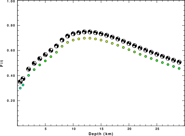
|
|
Figure 2. Depth sensitivity for waveform mechanism
|
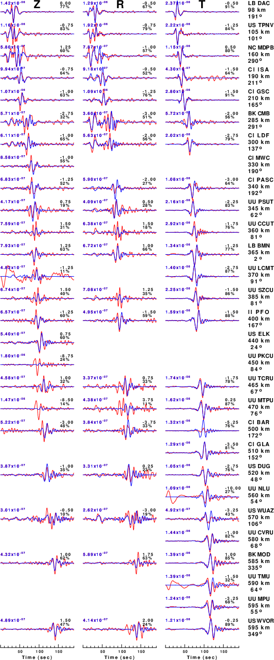
The comparison of the observed and predicted waveforms is given in the next figure. The red traces are the observed and the blue are the predicted.
Each observed-predicted component is plotted to the same scale and peak amplitudes are indicated by the numbers to the left of each trace. A pair of numbers is given in black at the right of each predicted traces. The upper number it the time shift required for maximum correlation between the observed and predicted traces. This time shift is required because the synthetics are not computed at exactly the same distance as the observed, the velocity model used in the predictions may not be perfect and the epicentral parameters may be be off.
A positive time shift indicates that the prediction is too fast and should be delayed to match the observed trace (shift to the right in this figure). A negative value indicates that the prediction is too slow. The lower number gives the percentage of variance reduction to characterize the individual goodness of fit (100% indicates a perfect fit).
The bandpass filter used in the processing and for the display was
hp c 0.02 n 3
lp c 0.06 n 3
|
|
Figure 3. Waveform comparison for selected depth. Red: observed; Blue - predicted. The time shift with respect to the model prediction is indicated. The percent of fit is also indicated. The time scale is relative to the first trace sample.
|
|
|
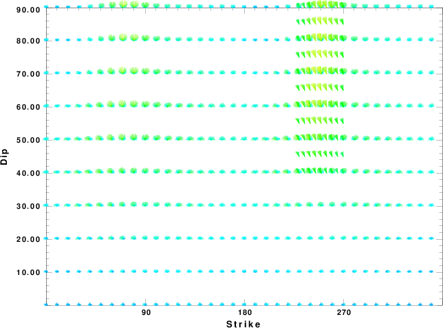
Focal mechanism sensitivity at the preferred depth. The red color indicates a very good fit to the waveforms.
Each solution is plotted as a vector at a given value of strike and dip with the angle of the vector representing the rake angle, measured, with respect to the upward vertical (N) in the figure.
|
A check on the assumed source location is possible by looking at the time shifts between the observed and predicted traces. The time shifts for waveform matching arise for several reasons:
- The origin time and epicentral distance are incorrect
- The velocity model used for the inversion is incorrect
- The velocity model used to define the P-arrival time is not the
same as the velocity model used for the waveform inversion
(assuming that the initial trace alignment is based on the
P arrival time)
Assuming only a mislocation, the time shifts are fit to a functional form:
Time_shift = A + B cos Azimuth + C Sin Azimuth
The time shifts for this inversion lead to the next figure:
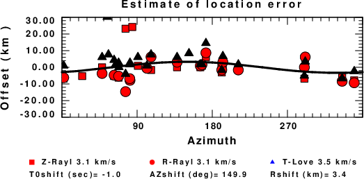
The derived shift in origin time and epicentral coordinates are given at the bottom of the figure.
Velocity Model
The WUS.model used for the waveform synthetic seismograms and for the surface wave eigenfunctions and dispersion is as follows
(The format is in the model96 format of Computer Programs in Seismology).
MODEL.01
Model after     8 iterations
ISOTROPIC
KGS
FLAT EARTH
1-D
CONSTANT VELOCITY
LINE08
LINE09
LINE10
LINE11
      H(KM)   VP(KM/S)   VS(KM/S) RHO(GM/CC)         QP         QS       ETAP       ETAS      FREFP      FREFS
     1.9000     3.4065     2.0089     2.2150  0.302E-02  0.679E-02   0.00       0.00       1.00       1.00
     6.1000     5.5445     3.2953     2.6089  0.349E-02  0.784E-02   0.00       0.00       1.00       1.00
    13.0000     6.2708     3.7396     2.7812  0.212E-02  0.476E-02   0.00       0.00       1.00       1.00
    19.0000     6.4075     3.7680     2.8223  0.111E-02  0.249E-02   0.00       0.00       1.00       1.00
     0.0000     7.9000     4.6200     3.2760  0.164E-10  0.370E-10   0.00       0.00       1.00       1.00
Last Changed Sat Apr 27 01:56:41 PM CDT 2024