Location
Location ANSS
The ANSS event ID is ak010cbf7et6 and the event page is at
https://earthquake.usgs.gov/earthquakes/eventpage/ak010cbf7et6/executive.
2010/09/25 12:06:00 62.854 -149.512 83.8 5.4 Alaska
Focal Mechanism
 USGS/SLU Moment Tensor Solution
 ENS  2010/09/25 12:06:00:0  62.85 -149.51  83.8 5.4 Alaska

 Stations used:
   AK.BMR AK.BPAW AK.BRLK AK.BWN AK.CCB AK.CHUM AK.CNP AK.DHY
   AK.DIV AK.DOT AK.EYAK AK.FIB AK.GLI AK.HDA AK.KLU AK.MCK
   AK.MDM AK.MLY AK.PAX AK.RC01 AK.RND AK.SAW AK.SCM AK.SKN
   AK.SSN AK.TRF AK.WRH IU.COLA

 Filtering commands used:
   hp c 0.02 n 3
   lp c 0.10 n 3

 Best Fitting Double Couple
  Mo = 1.43e+24 dyne-cm
  Mw = 5.37
  Z  = 89 km
  Plane   Strike  Dip  Rake
   NP1        7    69   148
   NP2      110    60    25
  Principal Axes:
   Axis    Value   Plunge  Azimuth
    T   1.43e+24     38     326
    N   0.00e+00     52     157
    P  -1.43e+24      5      60

 Moment Tensor: (dyne-cm)
    Component   Value
       Mxx     2.59e+23
       Mxy    -1.03e+24
       Mxz     5.05e+23
       Myy    -7.82e+23
       Myz    -5.05e+23
       Mzz     5.23e+23


                     ##########----
                 ###############-------
              ###################---------
             ####################----------
           ########   ###########-----------
          ######### T ############---------- P
         ##########   ############----------
        -#########################--------------
        --########################--------------
       ----#######################---------------
       ------#####################---------------
       -------###################----------------
       ----------################----------------
        ------------#############---------------
        ----------------########----------------
         --------------------###-------------##
          ---------------------###############
           --------------------##############
             -----------------#############
              ---------------#############
                 -----------###########
                     ------########


 Global CMT Convention Moment Tensor:
      R          T          P
  5.23e+23   5.05e+23   5.05e+23
  5.05e+23   2.59e+23   1.03e+24
  5.05e+23   1.03e+24  -7.82e+23


Details of the solution is found at

http://www.eas.slu.edu/eqc/eqc_mt/MECH.NA/20100925120600/index.html
|
Preferred Solution
The preferred solution from an analysis of the surface-wave spectral amplitude radiation pattern, waveform inversion or first motion observations is
      STK = 110
      DIP = 60
     RAKE = 25
       MW = 5.37
       HS = 89.0
The NDK file is 20100925120600.ndk
The waveform inversion is preferred.
Moment Tensor Comparison
The following compares this source inversion to those provided by others. The purpose is to look for major differences and also to note slight differences that might be inherent to the processing procedure. For completeness the USGS/SLU solution is repeated from above.
| SLU |
USGSMT |
 USGS/SLU Moment Tensor Solution
 ENS  2010/09/25 12:06:00:0  62.85 -149.51  83.8 5.4 Alaska

 Stations used:
   AK.BMR AK.BPAW AK.BRLK AK.BWN AK.CCB AK.CHUM AK.CNP AK.DHY
   AK.DIV AK.DOT AK.EYAK AK.FIB AK.GLI AK.HDA AK.KLU AK.MCK
   AK.MDM AK.MLY AK.PAX AK.RC01 AK.RND AK.SAW AK.SCM AK.SKN
   AK.SSN AK.TRF AK.WRH IU.COLA

 Filtering commands used:
   hp c 0.02 n 3
   lp c 0.10 n 3

 Best Fitting Double Couple
  Mo = 1.43e+24 dyne-cm
  Mw = 5.37
  Z  = 89 km
  Plane   Strike  Dip  Rake
   NP1        7    69   148
   NP2      110    60    25
  Principal Axes:
   Axis    Value   Plunge  Azimuth
    T   1.43e+24     38     326
    N   0.00e+00     52     157
    P  -1.43e+24      5      60

 Moment Tensor: (dyne-cm)
    Component   Value
       Mxx     2.59e+23
       Mxy    -1.03e+24
       Mxz     5.05e+23
       Myy    -7.82e+23
       Myz    -5.05e+23
       Mzz     5.23e+23


                     ##########----
                 ###############-------
              ###################---------
             ####################----------
           ########   ###########-----------
          ######### T ############---------- P
         ##########   ############----------
        -#########################--------------
        --########################--------------
       ----#######################---------------
       ------#####################---------------
       -------###################----------------
       ----------################----------------
        ------------#############---------------
        ----------------########----------------
         --------------------###-------------##
          ---------------------###############
           --------------------##############
             -----------------#############
              ---------------#############
                 -----------###########
                     ------########


 Global CMT Convention Moment Tensor:
      R          T          P
  5.23e+23   5.05e+23   5.05e+23
  5.05e+23   2.59e+23   1.03e+24
  5.05e+23   1.03e+24  -7.82e+23


Details of the solution is found at

http://www.eas.slu.edu/eqc/eqc_mt/MECH.NA/20100925120600/index.html
|
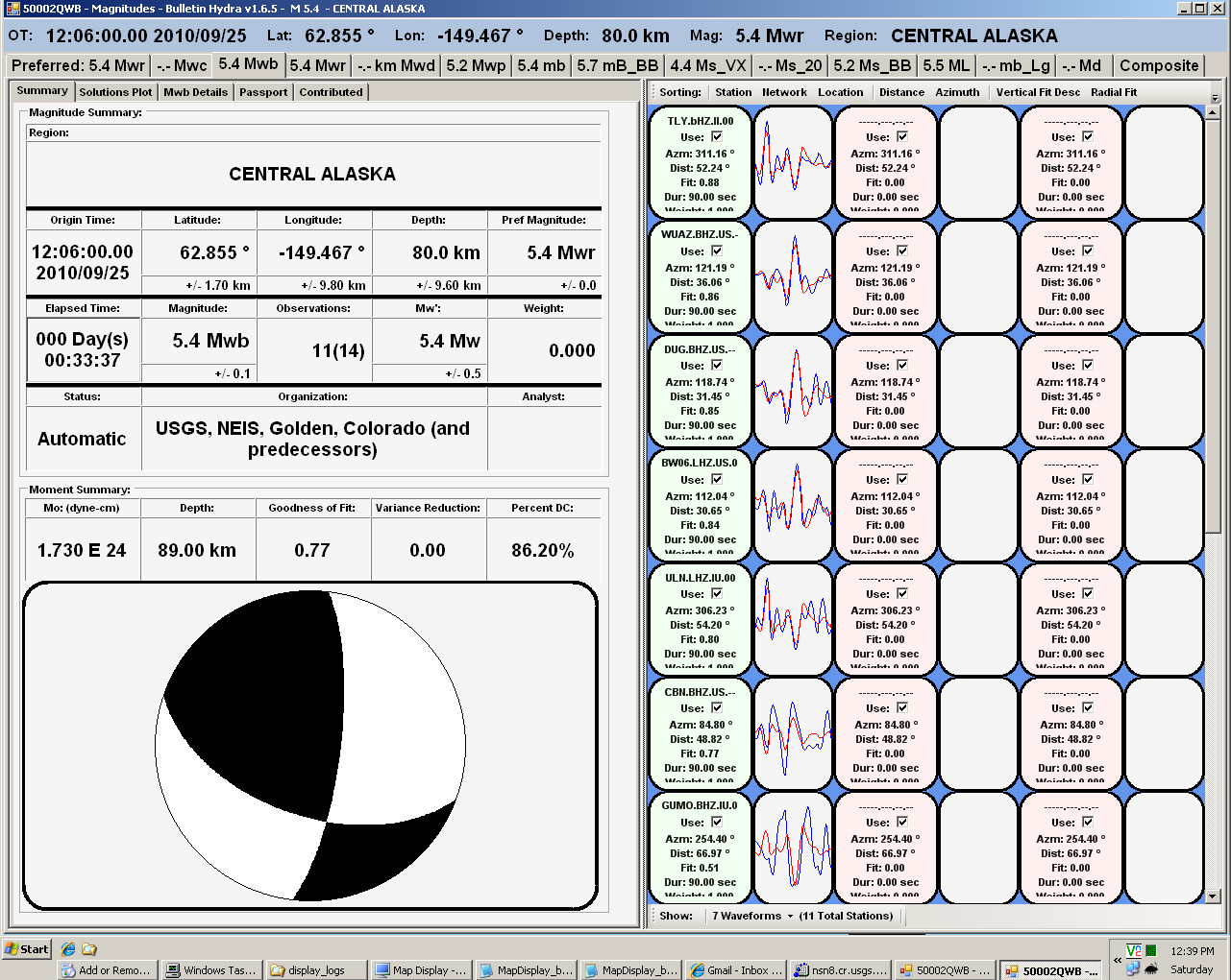
USGS Body-Wave Moment Tensor Solution

 10/09/25 12:06:00.00
 CENTRAL ALASKA
 Epicenter:  62.855 -149.467
 MW 5.4

 USGS MOMENT TENSOR SOLUTION
 Depth  89         No. of sta: 11
 Moment Tensor;   Scale 10**17 Nm
   Mrr= 0.53       Mtt= 0.29
   Mpp=-0.82       Mrt= 0.57
   Mrp= 0.87       Mtp= 1.18
  Principal axes:
   T  Val=  1.79  Plg=38  Azm=322
   N       -0.12      49      168
   P       -1.67      13       62

 Best Double Couple:Mo=1.7*10**17
  NP1:Strike=  7 Dip=74 Slip= 142
  NP2:       109     53        20

               ######-
          ###########------
        #############--------
      ################---------
    #######   ########--------
   ######## T ########-------- P -
   ########   ########--------   -
  -###################-------------
  ---#################-------------
  ----################-------------
  ------#############--------------
  ---------##########--------------
   -----------#######-------------
   ----------------#----------####
    ----------------#############
      -------------############
        ----------###########
          --------#########
               --#####
|
|
|
|
Magnitudes
Given the availability of digital waveforms for determination of the moment tensor, this section documents the added processing leading to mLg, if appropriate to the region, and ML by application of the respective IASPEI formulae. As a research study, the linear distance term of the IASPEI formula
for ML is adjusted to remove a linear distance trend in residuals to give a regionally defined ML. The defined ML uses horizontal component recordings, but the same procedure is applied to the vertical components since there may be some interest in vertical component ground motions. Residual plots versus distance may indicate interesting features of ground motion scaling in some distance ranges. A residual plot of the regionalized magnitude is given as a function of distance and azimuth, since data sets may transcend different wave propagation provinces.
mLg Magnitude
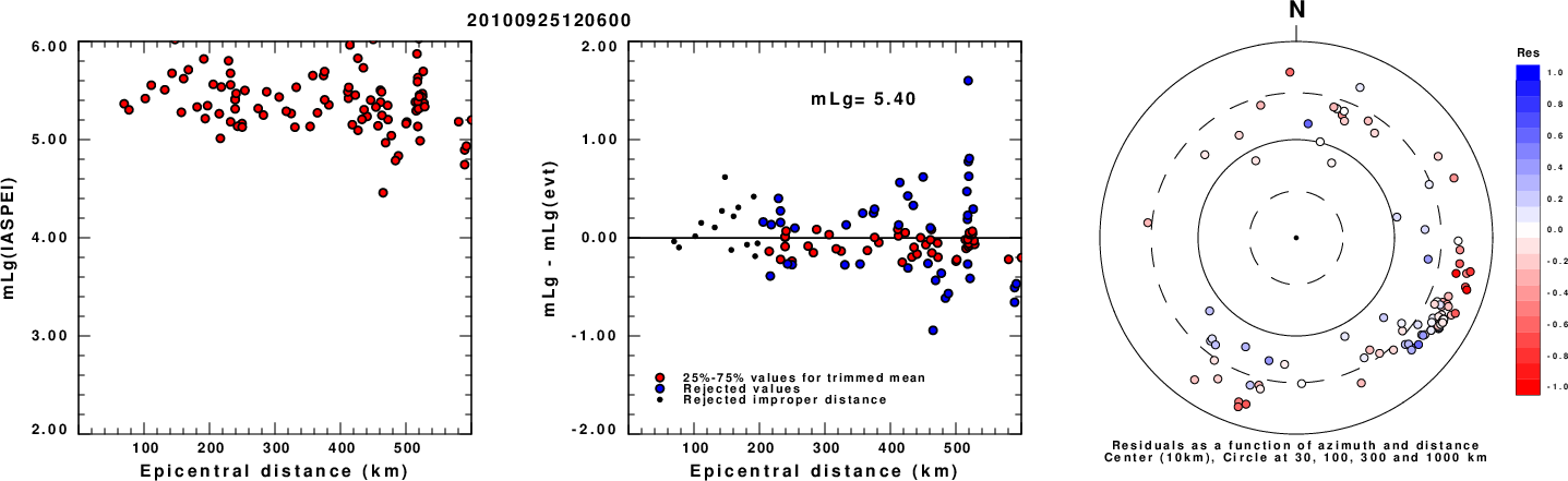
Left: mLg computed using the IASPEI formula. Center: mLg residuals versus epicentral distance ; the values used for the trimmed mean magnitude estimate are indicated.
Right: residuals as a function of distance and azimuth.
ML Magnitude
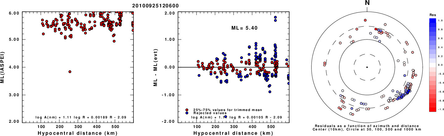
Left: ML computed using the IASPEI formula for Horizontal components. Center: ML residuals computed using a modified IASPEI formula that accounts for path specific attenuation; the values used for the trimmed mean are indicated. The ML relation used for each figure is given at the bottom of each plot.
Right: Residuals from new relation as a function of distance and azimuth.
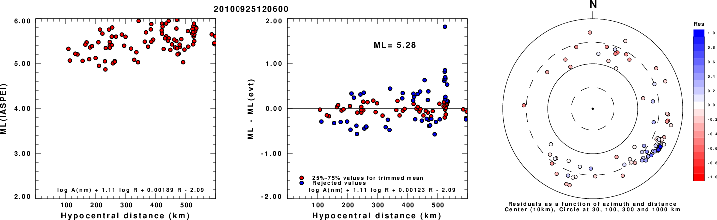
Left: ML computed using the IASPEI formula for Vertical components (research). Center: ML residuals computed using a modified IASPEI formula that accounts for path specific attenuation; the values used for the trimmed mean are indicated. The ML relation used for each figure is given at the bottom of each plot.
Right: Residuals from new relation as a function of distance and azimuth.
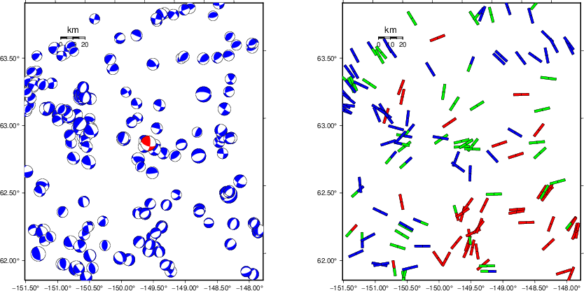
Context
The left panel of the next figure presents the focal mechanism for this earthquake (red) in the context of other nearby events (blue) in the SLU Moment Tensor Catalog. The right panel shows the inferred direction of maximum compressive stress and the type of faulting (green is strike-slip, red is normal, blue is thrust; oblique is shown by a combination of colors). Thus context plot is useful for assessing the appropriateness of the moment tensor of this event.
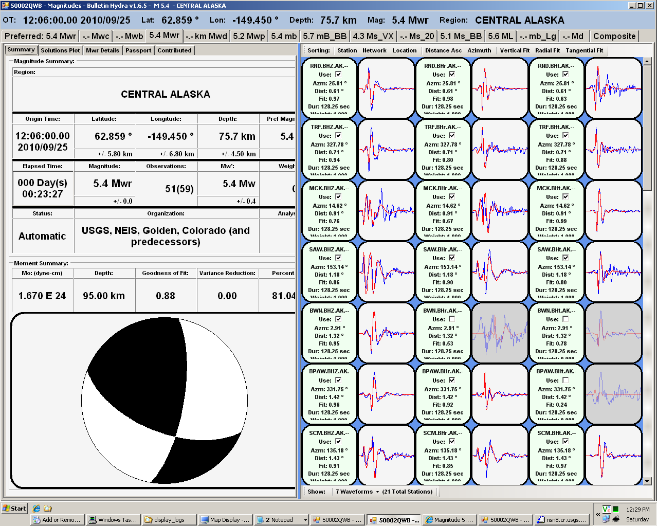
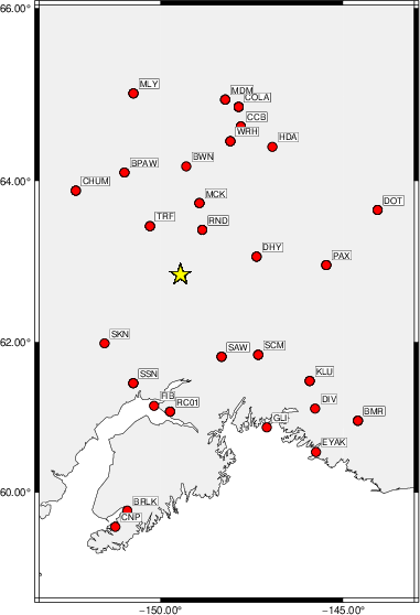
Waveform Inversion using wvfgrd96
The focal mechanism was determined using broadband seismic waveforms. The location of the event (star) and the
stations used for (red) the waveform inversion are shown in the next figure.
|
|
Location of broadband stations used for waveform inversion
|
The program wvfgrd96 was used with good traces observed at short distance to determine the focal mechanism, depth and seismic moment. This technique requires a high quality signal and well determined velocity model for the Green's functions. To the extent that these are the quality data, this type of mechanism should be preferred over the radiation pattern technique which requires the separate step of defining the pressure and tension quadrants and the correct strike.
The observed and predicted traces are filtered using the following gsac commands:
hp c 0.02 n 3
lp c 0.10 n 3
The results of this grid search are as follow:
           DEPTH  STK   DIP  RAKE   MW    FIT
WVFGRD96   60.0   105    50    20   5.30 0.4494
WVFGRD96   61.0   105    50    20   5.30 0.4586
WVFGRD96   62.0   110    50    25   5.31 0.4669
WVFGRD96   63.0   110    50    25   5.31 0.4761
WVFGRD96   64.0   110    50    25   5.32 0.4832
WVFGRD96   65.0   110    50    25   5.32 0.4916
WVFGRD96   66.0   110    50    25   5.32 0.4980
WVFGRD96   67.0   110    50    25   5.33 0.5032
WVFGRD96   68.0   110    50    25   5.33 0.5106
WVFGRD96   69.0   110    55    25   5.33 0.5163
WVFGRD96   70.0   110    55    25   5.33 0.5214
WVFGRD96   71.0   110    55    25   5.34 0.5289
WVFGRD96   72.0   110    55    25   5.34 0.5342
WVFGRD96   73.0   110    55    25   5.34 0.5383
WVFGRD96   74.0   110    55    25   5.34 0.5430
WVFGRD96   75.0   110    55    25   5.35 0.5466
WVFGRD96   76.0   110    55    25   5.35 0.5499
WVFGRD96   77.0   110    55    25   5.35 0.5531
WVFGRD96   78.0   110    55    25   5.35 0.5554
WVFGRD96   79.0   110    55    25   5.36 0.5568
WVFGRD96   80.0   110    55    25   5.36 0.5596
WVFGRD96   81.0   110    55    20   5.36 0.5597
WVFGRD96   82.0   110    55    20   5.37 0.5618
WVFGRD96   83.0   110    60    25   5.36 0.5629
WVFGRD96   84.0   110    60    25   5.36 0.5639
WVFGRD96   85.0   110    60    25   5.36 0.5661
WVFGRD96   86.0   110    60    25   5.36 0.5656
WVFGRD96   87.0   110    60    25   5.36 0.5672
WVFGRD96   88.0   110    60    25   5.37 0.5674
WVFGRD96   89.0   110    60    25   5.37 0.5698
WVFGRD96   90.0   110    60    25   5.37 0.5657
WVFGRD96   91.0   110    60    25   5.37 0.5675
WVFGRD96   92.0   110    60    25   5.37 0.5667
WVFGRD96   93.0   110    60    25   5.37 0.5671
WVFGRD96   94.0   110    60    25   5.37 0.5669
WVFGRD96   95.0   110    60    25   5.37 0.5681
WVFGRD96   96.0   110    60    25   5.37 0.5616
WVFGRD96   97.0   110    60    25   5.37 0.5635
WVFGRD96   98.0   110    60    20   5.38 0.5617
WVFGRD96   99.0   110    60    20   5.38 0.5615
WVFGRD96  100.0   110    60    20   5.38 0.5603
WVFGRD96  101.0   110    60    20   5.39 0.5583
WVFGRD96  102.0   110    60    20   5.39 0.5555
WVFGRD96  103.0   110    60    20   5.39 0.5560
WVFGRD96  104.0   110    60    20   5.39 0.5540
WVFGRD96  105.0   110    60    20   5.39 0.5528
WVFGRD96  106.0   110    60    20   5.39 0.5498
WVFGRD96  107.0   110    60    20   5.39 0.5481
WVFGRD96  108.0   110    60    20   5.39 0.5468
WVFGRD96  109.0   110    60    20   5.39 0.5449
WVFGRD96  110.0   110    60    20   5.39 0.5431
WVFGRD96  111.0   110    60    20   5.39 0.5398
WVFGRD96  112.0   110    60    20   5.39 0.5378
WVFGRD96  113.0   110    60    20   5.39 0.5361
WVFGRD96  114.0   110    65    20   5.39 0.5351
WVFGRD96  115.0   110    65    20   5.39 0.5313
WVFGRD96  116.0   110    65    20   5.39 0.5305
WVFGRD96  117.0   110    65    20   5.39 0.5287
WVFGRD96  118.0   110    65    20   5.39 0.5263
WVFGRD96  119.0   110    65    20   5.39 0.5255
WVFGRD96  120.0   110    65    20   5.39 0.5225
WVFGRD96  121.0   110    65    20   5.39 0.5209
WVFGRD96  122.0   110    65    20   5.39 0.5191
WVFGRD96  123.0   110    65    20   5.40 0.5165
WVFGRD96  124.0   110    65    20   5.40 0.5146
WVFGRD96  125.0   110    65    20   5.40 0.5130
WVFGRD96  126.0   110    65    20   5.40 0.5099
WVFGRD96  127.0   110    65    20   5.40 0.5097
WVFGRD96  128.0   110    65    20   5.40 0.5055
WVFGRD96  129.0   110    65    20   5.40 0.5050
The best solution is
WVFGRD96 89.0 110 60 25 5.37 0.5698
The mechanism corresponding to the best fit is
|
|
Figure 1. Waveform inversion focal mechanism
|
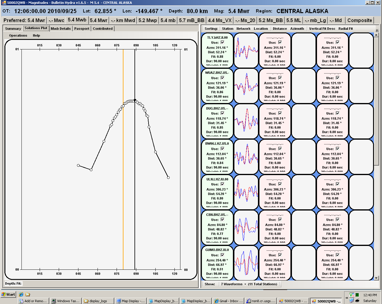
The best fit as a function of depth is given in the following figure:
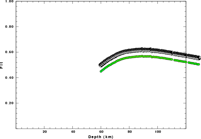
|
|
Figure 2. Depth sensitivity for waveform mechanism
|
The comparison of the observed and predicted waveforms is given in the next figure. The red traces are the observed and the blue are the predicted.
Each observed-predicted component is plotted to the same scale and peak amplitudes are indicated by the numbers to the left of each trace. A pair of numbers is given in black at the right of each predicted traces. The upper number it the time shift required for maximum correlation between the observed and predicted traces. This time shift is required because the synthetics are not computed at exactly the same distance as the observed, the velocity model used in the predictions may not be perfect and the epicentral parameters may be be off.
A positive time shift indicates that the prediction is too fast and should be delayed to match the observed trace (shift to the right in this figure). A negative value indicates that the prediction is too slow. The lower number gives the percentage of variance reduction to characterize the individual goodness of fit (100% indicates a perfect fit).
The bandpass filter used in the processing and for the display was
hp c 0.02 n 3
lp c 0.10 n 3
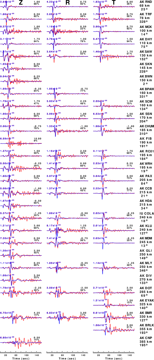
|
|
Figure 3. Waveform comparison for selected depth. Red: observed; Blue - predicted. The time shift with respect to the model prediction is indicated. The percent of fit is also indicated. The time scale is relative to the first trace sample.
|
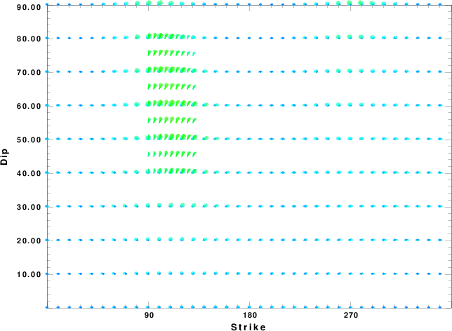
|
|
Focal mechanism sensitivity at the preferred depth. The red color indicates a very good fit to the waveforms.
Each solution is plotted as a vector at a given value of strike and dip with the angle of the vector representing the rake angle, measured, with respect to the upward vertical (N) in the figure.
|
A check on the assumed source location is possible by looking at the time shifts between the observed and predicted traces. The time shifts for waveform matching arise for several reasons:
- The origin time and epicentral distance are incorrect
- The velocity model used for the inversion is incorrect
- The velocity model used to define the P-arrival time is not the
same as the velocity model used for the waveform inversion
(assuming that the initial trace alignment is based on the
P arrival time)
Assuming only a mislocation, the time shifts are fit to a functional form:
Time_shift = A + B cos Azimuth + C Sin Azimuth
The time shifts for this inversion lead to the next figure:
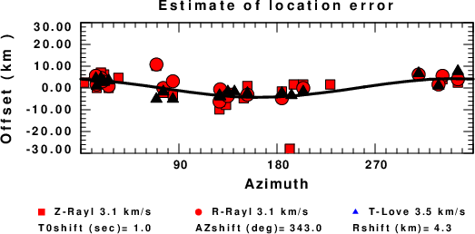
The derived shift in origin time and epicentral coordinates are given at the bottom of the figure.
Velocity Model
The WUS.model used for the waveform synthetic seismograms and for the surface wave eigenfunctions and dispersion is as follows
(The format is in the model96 format of Computer Programs in Seismology).
MODEL.01
Model after     8 iterations
ISOTROPIC
KGS
FLAT EARTH
1-D
CONSTANT VELOCITY
LINE08
LINE09
LINE10
LINE11
      H(KM)   VP(KM/S)   VS(KM/S) RHO(GM/CC)         QP         QS       ETAP       ETAS      FREFP      FREFS
     1.9000     3.4065     2.0089     2.2150  0.302E-02  0.679E-02   0.00       0.00       1.00       1.00
     6.1000     5.5445     3.2953     2.6089  0.349E-02  0.784E-02   0.00       0.00       1.00       1.00
    13.0000     6.2708     3.7396     2.7812  0.212E-02  0.476E-02   0.00       0.00       1.00       1.00
    19.0000     6.4075     3.7680     2.8223  0.111E-02  0.249E-02   0.00       0.00       1.00       1.00
     0.0000     7.9000     4.6200     3.2760  0.164E-10  0.370E-10   0.00       0.00       1.00       1.00
Last Changed Sat Apr 27 01:53:17 PM CDT 2024