Location

Location ANSS

The ANSS event ID is ak010c3azkox and the event page is at https://earthquake.usgs.gov/earthquakes/eventpage/ak010c3azkox/executive.

2010/09/20 21:24:24 61.115 -150.219 45.4 4.9 Alaska

Focal Mechanism

USGS/SLU Moment Tensor Solution ENS 2010/09/20 21:24:24:0 61.12 -150.22 45.4 4.9 Alaska Stations used: AK.BMR AK.BPAW AK.BRLK AK.CNP AK.CRQ AK.DHY AK.DIV AK.EYAK AK.FID AK.GLI AK.PAX AK.RAG AK.RC01 AK.RND AK.SAW AK.SCM AK.SKN AK.SSN AK.SWD AT.PMR AT.TTA Filtering commands used: hp c 0.02 n 3 lp c 0.08 n 3 Best Fitting Double Couple Mo = 2.07e+23 dyne-cm Mw = 4.81 Z = 48 km Plane Strike Dip Rake NP1 185 80 -85 NP2 338 11 -116 Principal Axes: Axis Value Plunge Azimuth T 2.07e+23 35 271 N 0.00e+00 5 4 P -2.07e+23 55 101 Moment Tensor: (dyne-cm) Component Value Mxx -2.54e+21 Mxy 1.13e+22 Mxz 2.00e+22 Myy 7.29e+22 Myz -1.92e+23 Mzz -7.04e+22 ########--#### ############-------### ##############-----------### ###############-------------## ################---------------### #################-----------------## #################-------------------## ##################-------------------### ##################--------------------## ###### ##########--------------------### ###### T ##########--------- ---------## ###### #########---------- P ---------## ##################---------- ---------## #################---------------------## #################---------------------## ################--------------------## ###############--------------------# ##############-------------------# ############-----------------# ###########----------------# #########------------# #####--------- Global CMT Convention Moment Tensor: R T P -7.04e+22 2.00e+22 1.92e+23 2.00e+22 -2.54e+21 -1.13e+22 1.92e+23 -1.13e+22 7.29e+22 Details of the solution is found at http://www.eas.slu.edu/eqc/eqc_mt/MECH.NA/20100920212424/index.html

Preferred Solution

      STK = 185
      DIP = 80
     RAKE = -85
       MW = 4.81
       HS = 48.0

The NDK file is 20100920212424.ndk The waveform inversion is preferred.

Moment Tensor Comparison

The following compares this source inversion to those provided by others. The purpose is to look for major differences and also to note slight differences that might be inherent to the processing procedure. For completeness the USGS/SLU solution is repeated from above.

SLU	USGSMT	AEIC
USGS/SLU Moment Tensor Solution ENS 2010/09/20 21:24:24:0 61.12 -150.22 45.4 4.9 Alaska Stations used: AK.BMR AK.BPAW AK.BRLK AK.CNP AK.CRQ AK.DHY AK.DIV AK.EYAK AK.FID AK.GLI AK.PAX AK.RAG AK.RC01 AK.RND AK.SAW AK.SCM AK.SKN AK.SSN AK.SWD AT.PMR AT.TTA Filtering commands used: hp c 0.02 n 3 lp c 0.08 n 3 Best Fitting Double Couple Mo = 2.07e+23 dyne-cm Mw = 4.81 Z = 48 km Plane Strike Dip Rake NP1 185 80 -85 NP2 338 11 -116 Principal Axes: Axis Value Plunge Azimuth T 2.07e+23 35 271 N 0.00e+00 5 4 P -2.07e+23 55 101 Moment Tensor: (dyne-cm) Component Value Mxx -2.54e+21 Mxy 1.13e+22 Mxz 2.00e+22 Myy 7.29e+22 Myz -1.92e+23 Mzz -7.04e+22 ########--#### ############-------### ##############-----------### ###############-------------## ################---------------### #################-----------------## #################-------------------## ##################-------------------### ##################--------------------## ###### ##########--------------------### ###### T ##########--------- ---------## ###### #########---------- P ---------## ##################---------- ---------## #################---------------------## #################---------------------## ################--------------------## ###############--------------------# ##############-------------------# ############-----------------# ###########----------------# #########------------# #####--------- Global CMT Convention Moment Tensor: R T P -7.04e+22 2.00e+22 1.92e+23 2.00e+22 -2.54e+21 -1.13e+22 1.92e+23 -1.13e+22 7.29e+22 Details of the solution is found at http://www.eas.slu.edu/eqc/eqc_mt/MECH.NA/20100920212424/index.html		Moment tensor inversion summary for event 2010/09/20 21:24 Date: 2010/09/20 Time: 21:24 (UTC) Region: Cook Inlet Region of Alaska Mw=4.8 Location: Lat. 61.1293; Lon. -150.2360; Depth 30 km (Best-fitting depth from moment tensor inversion) Solution quality: good; Number of stations = 9 Best Double Couple: strike dip rake Plane 1: 181.2 83.9 -93.7 Plane 2: 32.7 7.2 -58.8 Moment Tensor Parameters: Mo = 1.97165e+23 dyn-cm Mxx = 0.12; Mxy = -0.13; Mxz = 0.01 Myy = 0.34; Myz = -1.87; Mzz = -0.46 Principal Axes: value azimuth plunge T: 1.85 274.60 38.77 N: 0.12 181.61 3.71 P: -1.97 87.02 50.99

Magnitudes

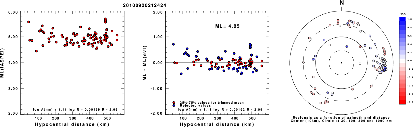
Given the availability of digital waveforms for determination of the moment tensor, this section documents the added processing leading to mLg, if appropriate to the region, and M_L by application of the respective IASPEI formulae. As a research study, the linear distance term of the IASPEI formula for M_L is adjusted to remove a linear distance trend in residuals to give a regionally defined M_L. The defined M_L uses horizontal component recordings, but the same procedure is applied to the vertical components since there may be some interest in vertical component ground motions. Residual plots versus distance may indicate interesting features of ground motion scaling in some distance ranges. A residual plot of the regionalized magnitude is given as a function of distance and azimuth, since data sets may transcend different wave propagation provinces.

ML Magnitude

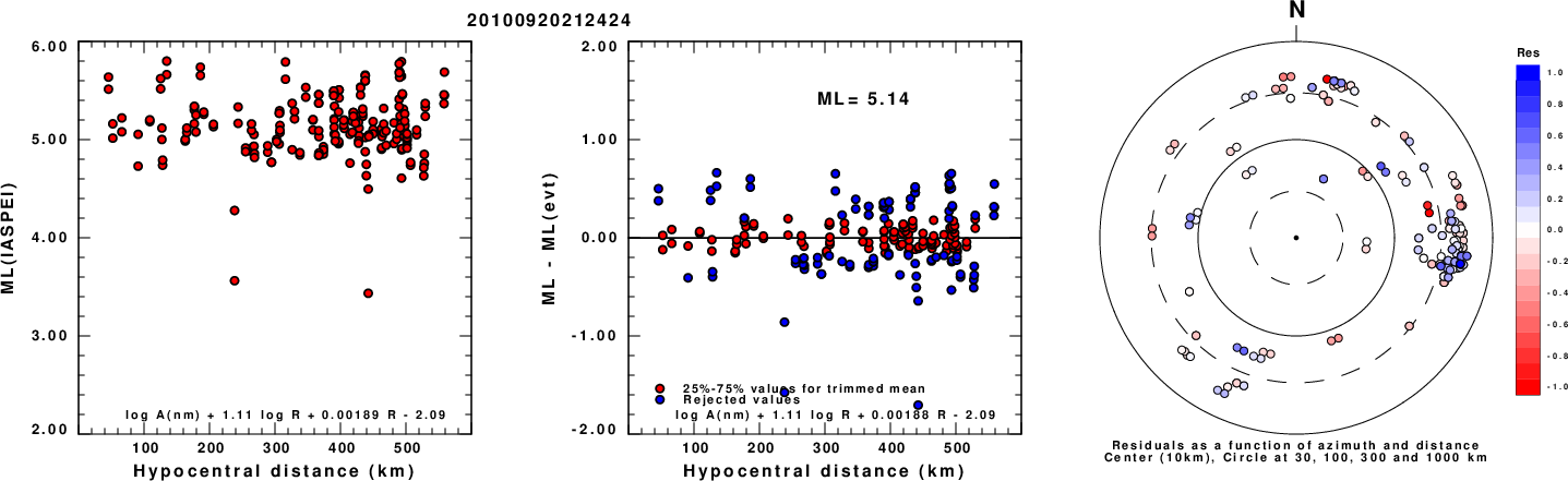
Left: ML computed using the IASPEI formula for Horizontal components. Center: ML residuals computed using a modified IASPEI formula that accounts for path specific attenuation; the values used for the trimmed mean are indicated. The ML relation used for each figure is given at the bottom of each plot. Right: Residuals from new relation as a function of distance and azimuth.

Left: ML computed using the IASPEI formula for Vertical components (research). Center: ML residuals computed using a modified IASPEI formula that accounts for path specific attenuation; the values used for the trimmed mean are indicated. The ML relation used for each figure is given at the bottom of each plot. Right: Residuals from new relation as a function of distance and azimuth.

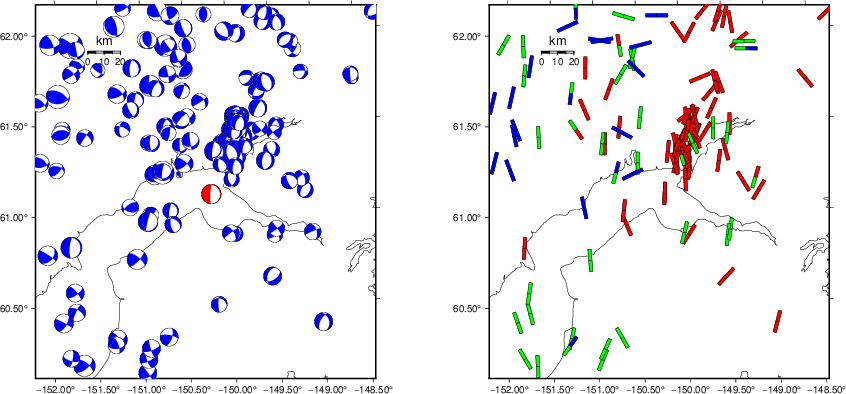
Context

Waveform Inversion using wvfgrd96

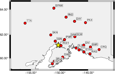
The focal mechanism was determined using broadband seismic waveforms. The location of the event (star) and the stations used for (red) the waveform inversion are shown in the next figure.

Location of broadband stations used for waveform inversion

The program wvfgrd96 was used with good traces observed at short distance to determine the focal mechanism, depth and seismic moment. This technique requires a high quality signal and well determined velocity model for the Green's functions. To the extent that these are the quality data, this type of mechanism should be preferred over the radiation pattern technique which requires the separate step of defining the pressure and tension quadrants and the correct strike.

The observed and predicted traces are filtered using the following gsac commands:

hp c 0.02 n 3
lp c 0.08 n 3

           DEPTH  STK   DIP  RAKE   MW    FIT
WVFGRD96   20.0    25    85    50   4.41 0.4667
WVFGRD96   21.0   200    90   -50   4.43 0.4786
WVFGRD96   22.0    25    85    50   4.44 0.4931
WVFGRD96   23.0    25    85    50   4.46 0.5058
WVFGRD96   24.0   205    90   -50   4.47 0.5178
WVFGRD96   25.0    25    90    55   4.48 0.5304
WVFGRD96   26.0    25    90    55   4.49 0.5421
WVFGRD96   27.0   200    85   -55   4.50 0.5532
WVFGRD96   28.0    10    90    60   4.51 0.5645
WVFGRD96   29.0    10    90    60   4.53 0.5772
WVFGRD96   30.0    10    90    60   4.54 0.5890
WVFGRD96   31.0    10    90    65   4.55 0.5999
WVFGRD96   32.0    10    90    65   4.56 0.6098
WVFGRD96   33.0   185    85   -65   4.57 0.6247
WVFGRD96   34.0   190    85   -70   4.58 0.6341
WVFGRD96   35.0   185    80   -70   4.58 0.6434
WVFGRD96   36.0   185    80   -70   4.59 0.6524
WVFGRD96   37.0   185    80   -70   4.60 0.6599
WVFGRD96   38.0   185    80   -70   4.60 0.6667
WVFGRD96   39.0   185    80   -70   4.61 0.6703
WVFGRD96   40.0   185    80   -80   4.75 0.6652
WVFGRD96   41.0   185    80   -80   4.76 0.6773
WVFGRD96   42.0   185    80   -80   4.77 0.6868
WVFGRD96   43.0   185    80   -80   4.78 0.6952
WVFGRD96   44.0   185    80   -80   4.78 0.7011
WVFGRD96   45.0   185    80   -80   4.79 0.7071
WVFGRD96   46.0   185    80   -80   4.80 0.7105
WVFGRD96   47.0   185    80   -80   4.80 0.7139
WVFGRD96   48.0   185    80   -85   4.81 0.7159
WVFGRD96   49.0   -10    10  -105   4.82 0.7151
WVFGRD96   50.0   -10    10  -105   4.83 0.7153
WVFGRD96   51.0   -10    10  -105   4.83 0.7143
WVFGRD96   52.0   -10    10  -105   4.84 0.7121
WVFGRD96   53.0   -10    10  -105   4.84 0.7092
WVFGRD96   54.0    50    15   -50   4.86 0.7049
WVFGRD96   55.0    50    15   -50   4.87 0.7032
WVFGRD96   56.0    50    15   -50   4.87 0.6999
WVFGRD96   57.0    50    15   -50   4.88 0.6959
WVFGRD96   58.0    50    15   -50   4.88 0.6916
WVFGRD96   59.0    50    15   -50   4.88 0.6856

The best solution is

WVFGRD96   48.0   185    80   -85   4.81 0.7159

The mechanism corresponding to the best fit is

Figure 1. Waveform inversion focal mechanism

The best fit as a function of depth is given in the following figure:

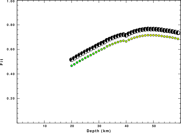
Figure 2. Depth sensitivity for waveform mechanism

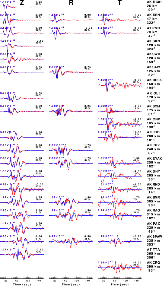
The comparison of the observed and predicted waveforms is given in the next figure. The red traces are the observed and the blue are the predicted. Each observed-predicted component is plotted to the same scale and peak amplitudes are indicated by the numbers to the left of each trace. A pair of numbers is given in black at the right of each predicted traces. The upper number it the time shift required for maximum correlation between the observed and predicted traces. This time shift is required because the synthetics are not computed at exactly the same distance as the observed, the velocity model used in the predictions may not be perfect and the epicentral parameters may be be off. A positive time shift indicates that the prediction is too fast and should be delayed to match the observed trace (shift to the right in this figure). A negative value indicates that the prediction is too slow. The lower number gives the percentage of variance reduction to characterize the individual goodness of fit (100% indicates a perfect fit).

The bandpass filter used in the processing and for the display was

hp c 0.02 n 3
lp c 0.08 n 3

Figure 3. Waveform comparison for selected depth. Red: observed; Blue - predicted. The time shift with respect to the model prediction is indicated. The percent of fit is also indicated. The time scale is relative to the first trace sample.

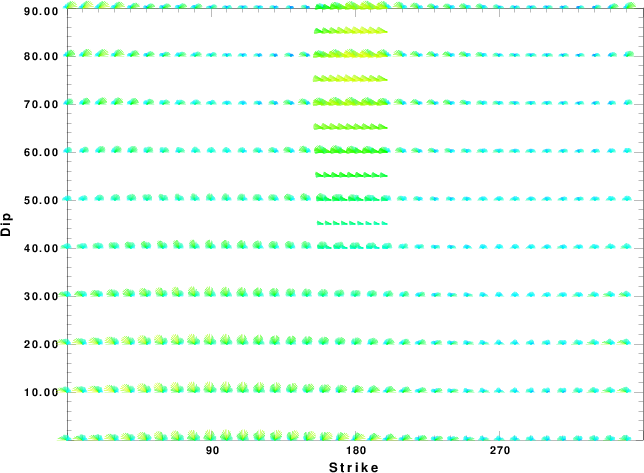
Focal mechanism sensitivity at the preferred depth. The red color indicates a very good fit to the waveforms. Each solution is plotted as a vector at a given value of strike and dip with the angle of the vector representing the rake angle, measured, with respect to the upward vertical (N) in the figure.

A check on the assumed source location is possible by looking at the time shifts between the observed and predicted traces. The time shifts for waveform matching arise for several reasons:

• The origin time and epicentral distance are incorrect
• The velocity model used for the inversion is incorrect
• The velocity model used to define the P-arrival time is not the same as the velocity model used for the waveform inversion (assuming that the initial trace alignment is based on the P arrival time)

 Time_shift = A + B cos Azimuth + C Sin Azimuth

The time shifts for this inversion lead to the next figure:

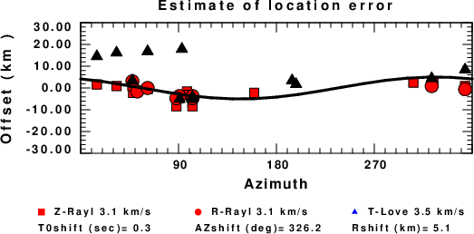
The derived shift in origin time and epicentral coordinates are given at the bottom of the figure.

Velocity Model

The WUS.model used for the waveform synthetic seismograms and for the surface wave eigenfunctions and dispersion is as follows (The format is in the model96 format of Computer Programs in Seismology).

MODEL.01
Model after     8 iterations
ISOTROPIC
KGS
FLAT EARTH
1-D
CONSTANT VELOCITY
LINE08
LINE09
LINE10
LINE11
      H(KM)   VP(KM/S)   VS(KM/S) RHO(GM/CC)         QP         QS       ETAP       ETAS      FREFP      FREFS
     1.9000     3.4065     2.0089     2.2150  0.302E-02  0.679E-02   0.00       0.00       1.00       1.00    
     6.1000     5.5445     3.2953     2.6089  0.349E-02  0.784E-02   0.00       0.00       1.00       1.00    
    13.0000     6.2708     3.7396     2.7812  0.212E-02  0.476E-02   0.00       0.00       1.00       1.00    
    19.0000     6.4075     3.7680     2.8223  0.111E-02  0.249E-02   0.00       0.00       1.00       1.00    
     0.0000     7.9000     4.6200     3.2760  0.164E-10  0.370E-10   0.00       0.00       1.00       1.00