Location
SLU Location
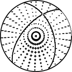
To check the ANSS location or to compare the observed P-wave first motions to the moment tensor solution, P- and S-wave first arrival times were manually read together with the P-wave first motions. The subsequent output of the program elocate is given in the file elocate.txt. The first motion plot is shown below.
Location ANSS
The ANSS event ID is usp000h7ax and the event page is at
https://earthquake.usgs.gov/earthquakes/eventpage/usp000h7ax/executive.
2010/02/15 03:32:25 35.557 -97.298 3.3 3.0 Oklahoma
Focal Mechanism
 USGS/SLU Moment Tensor Solution
 ENS  2010/02/15 03:32:25:0  35.56  -97.30   3.3 3.0 Oklahoma

 Stations used:
   GS.OK001 GS.OK003 GS.OK004 GS.OK005 GS.OK006 TA.V34A
   TA.W34A

 Filtering commands used:
   rtr
   hp c 0.5 n 3
   lp c 2.00 n 3
   br c 0.12 0.25 n 4 p 2

 Best Fitting Double Couple
  Mo = 5.82e+20 dyne-cm
  Mw = 3.11
  Z  = 7 km
  Plane   Strike  Dip  Rake
   NP1      222    61   132
   NP2      340    50    40
  Principal Axes:
   Axis    Value   Plunge  Azimuth
    T   5.82e+20     53     185
    N   0.00e+00     36      17
    P  -5.82e+20      6     283

 Moment Tensor: (dyne-cm)
    Component   Value
       Mxx     1.76e+20
       Mxy     1.43e+20
       Mxz    -2.92e+20
       Myy    -5.45e+20
       Myz     3.70e+19
       Mzz     3.68e+20


                     ##############
                 ---------#############
              ---------------#############
             ------------------###---------
           --------------------##------------
          ------------------######------------
         -----------------#########------------
          --------------############------------
        P ------------###############-----------
          -----------#################-----------
       ------------###################-----------
       -----------#####################----------
       ----------######################----------
        --------#######################---------
        -------###########   ##########---------
         ------########### T ##########--------
          ----############   ##########-------
           ---#########################------
             -########################-----
              #######################-----
                 ###################---
                     ##############


 Global CMT Convention Moment Tensor:
      R          T          P
  3.68e+20  -2.92e+20  -3.70e+19
 -2.92e+20   1.76e+20  -1.43e+20
 -3.70e+19  -1.43e+20  -5.45e+20


Details of the solution is found at

http://www.eas.slu.edu/eqc/eqc_mt/MECH.NA/20100215033225/index.html
|
Preferred Solution
The preferred solution from an analysis of the surface-wave spectral amplitude radiation pattern, waveform inversion or first motion observations is
      STK = 340
      DIP = 50
     RAKE = 40
       MW = 3.11
       HS = 7.0
The NDK file is 20100215033225.ndk
The waveform inversion is preferred.
Moment Tensor Comparison
The following compares this source inversion to those provided by others. The purpose is to look for major differences and also to note slight differences that might be inherent to the processing procedure. For completeness the USGS/SLU solution is repeated from above.
| SLU |
SLUFM |
 USGS/SLU Moment Tensor Solution
 ENS  2010/02/15 03:32:25:0  35.56  -97.30   3.3 3.0 Oklahoma

 Stations used:
   GS.OK001 GS.OK003 GS.OK004 GS.OK005 GS.OK006 TA.V34A
   TA.W34A

 Filtering commands used:
   rtr
   hp c 0.5 n 3
   lp c 2.00 n 3
   br c 0.12 0.25 n 4 p 2

 Best Fitting Double Couple
  Mo = 5.82e+20 dyne-cm
  Mw = 3.11
  Z  = 7 km
  Plane   Strike  Dip  Rake
   NP1      222    61   132
   NP2      340    50    40
  Principal Axes:
   Axis    Value   Plunge  Azimuth
    T   5.82e+20     53     185
    N   0.00e+00     36      17
    P  -5.82e+20      6     283

 Moment Tensor: (dyne-cm)
    Component   Value
       Mxx     1.76e+20
       Mxy     1.43e+20
       Mxz    -2.92e+20
       Myy    -5.45e+20
       Myz     3.70e+19
       Mzz     3.68e+20


                     ##############
                 ---------#############
              ---------------#############
             ------------------###---------
           --------------------##------------
          ------------------######------------
         -----------------#########------------
          --------------############------------
        P ------------###############-----------
          -----------#################-----------
       ------------###################-----------
       -----------#####################----------
       ----------######################----------
        --------#######################---------
        -------###########   ##########---------
         ------########### T ##########--------
          ----############   ##########-------
           ---#########################------
             -########################-----
              #######################-----
                 ###################---
                     ##############


 Global CMT Convention Moment Tensor:
      R          T          P
  3.68e+20  -2.92e+20  -3.70e+19
 -2.92e+20   1.76e+20  -1.43e+20
 -3.70e+19  -1.43e+20  -5.45e+20


Details of the solution is found at

http://www.eas.slu.edu/eqc/eqc_mt/MECH.NA/20100215033225/index.html
|
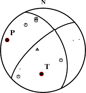
The first motion plot is not very satisfying. I plot the observed Z
components about the P-arrival pick. The takeoff angles and picks are
in the elocate.txt file. At these short distances there is sensitivity
of the take-off angles and azimuths to the location. The nodal planes
are sensitive to the distance weighting. So this may be an apparent
inconsistency in the comparison of observed and predicted first
motions.
|
Context
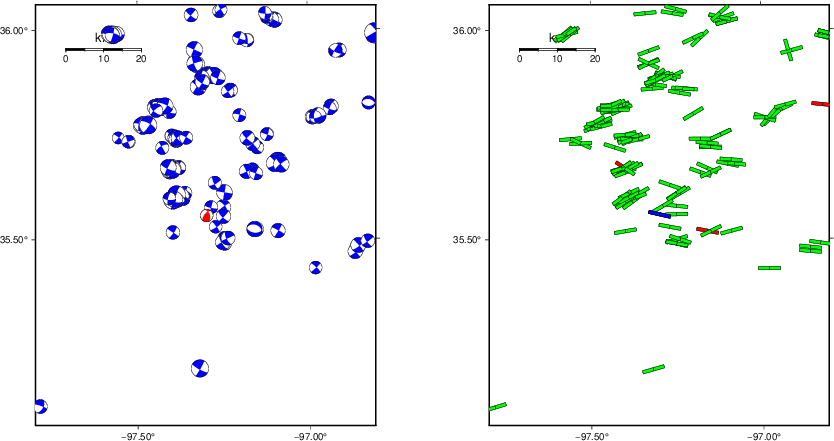
The left panel of the next figure presents the focal mechanism for this earthquake (red) in the context of other nearby events (blue) in the SLU Moment Tensor Catalog. The right panel shows the inferred direction of maximum compressive stress and the type of faulting (green is strike-slip, red is normal, blue is thrust; oblique is shown by a combination of colors). Thus context plot is useful for assessing the appropriateness of the moment tensor of this event.
Waveform Inversion using wvfgrd96
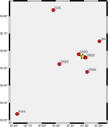
The focal mechanism was determined using broadband seismic waveforms. The location of the event (star) and the
stations used for (red) the waveform inversion are shown in the next figure.
|
|
Location of broadband stations used for waveform inversion
|
The program wvfgrd96 was used with good traces observed at short distance to determine the focal mechanism, depth and seismic moment. This technique requires a high quality signal and well determined velocity model for the Green's functions. To the extent that these are the quality data, this type of mechanism should be preferred over the radiation pattern technique which requires the separate step of defining the pressure and tension quadrants and the correct strike.
The observed and predicted traces are filtered using the following gsac commands:
rtr
hp c 0.5 n 3
lp c 2.00 n 3
br c 0.12 0.25 n 4 p 2
The results of this grid search are as follow:
           DEPTH  STK   DIP  RAKE   MW    FIT
WVFGRD96    0.5    55    75    25   2.08 0.1149
WVFGRD96    1.0    55    30   -20   2.22 0.1464
WVFGRD96    2.0    65    40     0   2.63 0.2466
WVFGRD96    3.0    45    50    75   2.73 0.2339
WVFGRD96    4.0   355    85   -30   2.96 0.3653
WVFGRD96    5.0   335    50    25   3.01 0.7015
WVFGRD96    6.0   335    50    30   3.06 0.6848
WVFGRD96    7.0   340    50    40   3.11 0.7090
WVFGRD96    8.0   340    50    45   3.16 0.5723
WVFGRD96    9.0   345    80    80   3.12 0.3753
WVFGRD96   10.0   345    80    75   3.14 0.3641
WVFGRD96   11.0   325    70   -75   3.04 0.1580
WVFGRD96   12.0   330    75   -70   3.03 0.1451
WVFGRD96   13.0   335    75   -70   2.97 0.0826
WVFGRD96   14.0    70    45    30   2.82 0.0251
WVFGRD96   15.0    70    50    25   2.84 0.0242
WVFGRD96   16.0    70    50    25   2.84 0.0214
WVFGRD96   17.0    20    80    30   2.83 0.0086
WVFGRD96   18.0   180    60   -30   2.82 0.0084
WVFGRD96   19.0   195    10    55   2.73 0.0077
WVFGRD96   20.0   190    65   -50   2.80 0.0073
WVFGRD96   21.0    20    40   -70   2.80 0.0059
WVFGRD96   22.0    30    45   -65   2.80 0.0055
WVFGRD96   23.0   295    65    45   2.80 0.0060
WVFGRD96   24.0     5    45   -30   2.84 0.0052
WVFGRD96   25.0   180    55    75   2.83 0.0054
WVFGRD96   26.0   175    55    65   2.86 0.0059
WVFGRD96   27.0   315    65   -60   2.77 0.0047
WVFGRD96   28.0   300    70   -55   2.85 0.0076
WVFGRD96   29.0   295    65   -50   2.89 0.0078
The best solution is
WVFGRD96 7.0 340 50 40 3.11 0.7090
The mechanism corresponding to the best fit is
|
|
Figure 1. Waveform inversion focal mechanism
|
The best fit as a function of depth is given in the following figure:
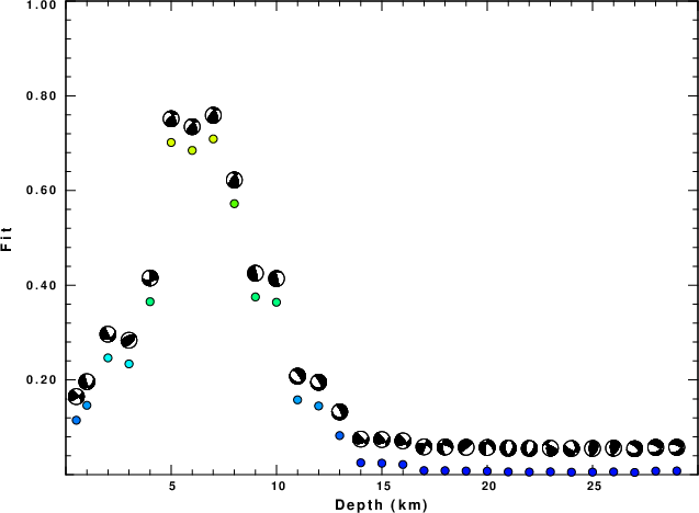
|
|
Figure 2. Depth sensitivity for waveform mechanism
|
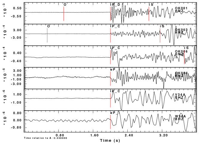
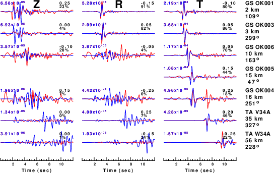
The comparison of the observed and predicted waveforms is given in the next figure. The red traces are the observed and the blue are the predicted.
Each observed-predicted component is plotted to the same scale and peak amplitudes are indicated by the numbers to the left of each trace. A pair of numbers is given in black at the right of each predicted traces. The upper number it the time shift required for maximum correlation between the observed and predicted traces. This time shift is required because the synthetics are not computed at exactly the same distance as the observed, the velocity model used in the predictions may not be perfect and the epicentral parameters may be be off.
A positive time shift indicates that the prediction is too fast and should be delayed to match the observed trace (shift to the right in this figure). A negative value indicates that the prediction is too slow. The lower number gives the percentage of variance reduction to characterize the individual goodness of fit (100% indicates a perfect fit).
The bandpass filter used in the processing and for the display was
rtr
hp c 0.5 n 3
lp c 2.00 n 3
br c 0.12 0.25 n 4 p 2
|
|
Figure 3. Waveform comparison for selected depth. Red: observed; Blue - predicted. The time shift with respect to the model prediction is indicated. The percent of fit is also indicated. The time scale is relative to the first trace sample.
|
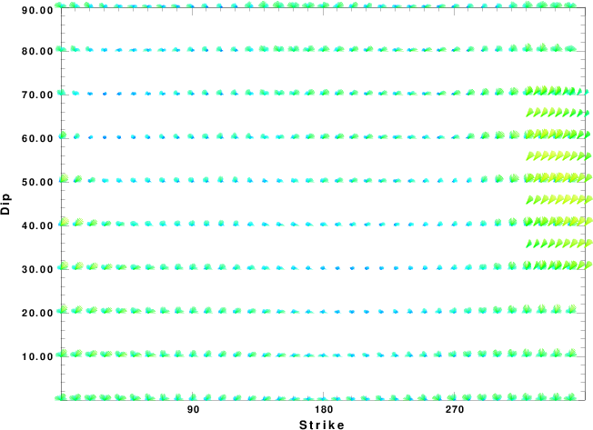
|
|
Focal mechanism sensitivity at the preferred depth. The red color indicates a very good fit to the waveforms.
Each solution is plotted as a vector at a given value of strike and dip with the angle of the vector representing the rake angle, measured, with respect to the upward vertical (N) in the figure.
|
A check on the assumed source location is possible by looking at the time shifts between the observed and predicted traces. The time shifts for waveform matching arise for several reasons:
- The origin time and epicentral distance are incorrect
- The velocity model used for the inversion is incorrect
- The velocity model used to define the P-arrival time is not the
same as the velocity model used for the waveform inversion
(assuming that the initial trace alignment is based on the
P arrival time)
Assuming only a mislocation, the time shifts are fit to a functional form:
Time_shift = A + B cos Azimuth + C Sin Azimuth
The time shifts for this inversion lead to the next figure:
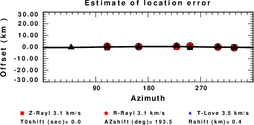
The derived shift in origin time and epicentral coordinates are given at the bottom of the figure.
Velocity Model
The WUS.model used for the waveform synthetic seismograms and for the surface wave eigenfunctions and dispersion is as follows
(The format is in the model96 format of Computer Programs in Seismology).
MODEL.01
Model after     8 iterations
ISOTROPIC
KGS
FLAT EARTH
1-D
CONSTANT VELOCITY
LINE08
LINE09
LINE10
LINE11
      H(KM)   VP(KM/S)   VS(KM/S) RHO(GM/CC)         QP         QS       ETAP       ETAS      FREFP      FREFS
     1.9000     3.4065     2.0089     2.2150  0.302E-02  0.679E-02   0.00       0.00       1.00       1.00
     6.1000     5.5445     3.2953     2.6089  0.349E-02  0.784E-02   0.00       0.00       1.00       1.00
    13.0000     6.2708     3.7396     2.7812  0.212E-02  0.476E-02   0.00       0.00       1.00       1.00
    19.0000     6.4075     3.7680     2.8223  0.111E-02  0.249E-02   0.00       0.00       1.00       1.00
     0.0000     7.9000     4.6200     3.2760  0.164E-10  0.370E-10   0.00       0.00       1.00       1.00
Last Changed Sat Apr 27 03:34:49 PM CDT 2024