The ANSS event ID is usp000h44s and the event page is at https://earthquake.usgs.gov/earthquakes/eventpage/usp000h44s/executive.
2009/11/17 15:30:46 52.123 -131.395 17.0 6.6 British Columbia
 USGS/SLU Moment Tensor Solution
 ENS  2009/11/17 15:30:46:0  52.12 -131.40  17.0 6.6 British Columbia

 Stations used:
   AK.BESE AT.CRAG AT.SIT AT.SKAG CN.BBB CN.CBB CN.DLBC CN.EDB
   CN.FNBB CN.HNB CN.HOPB CN.LLLB CN.NLLB CN.PGC CN.PHC CN.PNT
   CN.RUBB CN.SLEB CN.SNB CN.VGZ CN.YOUB UW.LON UW.LTY

 Filtering commands used:
   hp c 0.01 n 3
   lp c 0.025 n 3

 Best Fitting Double Couple
  Mo = 3.67e+25 dyne-cm
  Mw = 6.31
  Z  = 11 km
  Plane   Strike  Dip  Rake
   NP1      175    90   -170
   NP2       85    80     0
  Principal Axes:
   Axis    Value   Plunge  Azimuth
    T   3.67e+25      7     310
    N   0.00e+00     80     175
    P  -3.67e+25      7      40

 Moment Tensor: (dyne-cm)
    Component   Value
       Mxx    -6.28e+24
       Mxy    -3.56e+25
       Mxz    -5.56e+23
       Myy     6.28e+24
       Myz    -6.35e+24
       Mzz     0.00e+00


                     #####---------
                 #########-------------
              #############-------------
              #############------------- P
            T #############-------------   --
          #   #############-------------------
         ##################--------------------
        ###################---------------------
        ####################--------------------
       #####################---------------------
       #####################------------------###
       #####################------------#########
       -------###########---#####################
        --------------------####################
        ---------------------###################
         --------------------##################
          -------------------#################
           ------------------################
             ----------------##############
              ---------------#############
                 -------------#########
                     ---------#####


 Global CMT Convention Moment Tensor:
      R          T          P
  0.00e+00  -5.56e+23   6.35e+24
 -5.56e+23  -6.28e+24   3.56e+25
  6.35e+24   3.56e+25   6.28e+24


Details of the solution is found at

http://www.eas.slu.edu/eqc/eqc_mt/MECH.NA/20091117153046/index.html
|
      STK = 85
      DIP = 80
     RAKE = 0
       MW = 6.31
       HS = 11.0
The NDK file is 20091117153046.ndk The waveform inversion is preferred.
The following compares this source inversion to those provided by others. The purpose is to look for major differences and also to note slight differences that might be inherent to the processing procedure. For completeness the USGS/SLU solution is repeated from above.
 USGS/SLU Moment Tensor Solution
 ENS  2009/11/17 15:30:46:0  52.12 -131.40  17.0 6.6 British Columbia

 Stations used:
   AK.BESE AT.CRAG AT.SIT AT.SKAG CN.BBB CN.CBB CN.DLBC CN.EDB
   CN.FNBB CN.HNB CN.HOPB CN.LLLB CN.NLLB CN.PGC CN.PHC CN.PNT
   CN.RUBB CN.SLEB CN.SNB CN.VGZ CN.YOUB UW.LON UW.LTY

 Filtering commands used:
   hp c 0.01 n 3
   lp c 0.025 n 3

 Best Fitting Double Couple
  Mo = 3.67e+25 dyne-cm
  Mw = 6.31
  Z  = 11 km
  Plane   Strike  Dip  Rake
   NP1      175    90   -170
   NP2       85    80     0
  Principal Axes:
   Axis    Value   Plunge  Azimuth
    T   3.67e+25      7     310
    N   0.00e+00     80     175
    P  -3.67e+25      7      40

 Moment Tensor: (dyne-cm)
    Component   Value
       Mxx    -6.28e+24
       Mxy    -3.56e+25
       Mxz    -5.56e+23
       Myy     6.28e+24
       Myz    -6.35e+24
       Mzz     0.00e+00


                     #####---------
                 #########-------------
              #############-------------
              #############------------- P
            T #############-------------   --
          #   #############-------------------
         ##################--------------------
        ###################---------------------
        ####################--------------------
       #####################---------------------
       #####################------------------###
       #####################------------#########
       -------###########---#####################
        --------------------####################
        ---------------------###################
         --------------------##################
          -------------------#################
           ------------------################
             ----------------##############
              ---------------#############
                 -------------#########
                     ---------#####


 Global CMT Convention Moment Tensor:
      R          T          P
  0.00e+00  -5.56e+23   6.35e+24
 -5.56e+23  -6.28e+24   3.56e+25
  6.35e+24   3.56e+25   6.28e+24


Details of the solution is found at

http://www.eas.slu.edu/eqc/eqc_mt/MECH.NA/20091117153046/index.html
|
USGS Body-Wave Moment Tensor Solution

 09/11/17 15:30:46.03
 QUEEN CHARLOTTE ISLANDS REGION
 Epicenter:  52.093 -131.419
 MW 6.4

 USGS MOMENT TENSOR SOLUTION
 Depth  14         No. of sta: 81
 Moment Tensor;   Scale 10**18 Nm
   Mrr=-0.41       Mtt=-1.39
   Mpp= 1.79       Mrt= 0.33
   Mrp=-1.15       Mtp= 5.29
  Principal axes:
   T  Val=  5.81  Plg= 6  Azm=126
   N       -0.31      77        4
   P       -5.50      10      217

 Best Double Couple:Mo=5.7*10**18
  NP1:Strike=352 Dip=87 Slip=-168
  NP2:       261     78        -3

               #------
          #######----------
        #########------------
      ###########--------------
    ##############---------------
   ###############----------------
   ###############----------------
  ################-----------------
  #############----################
  ######-----------################
  #----------------################
  ------------------###############
   -----------------##############
   -----------------##########   #
    ----   ---------########## T
      -- P ---------##########
           ----------########
          -----------######
               ------#
|
November 17, 2009, QUEEN CHARLOTTE ISLANDS REGION, MW=6.6

Vala Hjorleifsdottir

CENTROID-MOMENT-TENSOR  SOLUTION
GCMT EVENT:     C200911171530A
DATA: II IU CU IC G  GE
L.P.BODY WAVES:112S, 261C, T= 50
MANTLE WAVES:  106S, 201C, T=125
SURFACE WAVES: 111S, 273C, T= 50
TIMESTAMP:      Q-20091117202117
CENTROID LOCATION:
ORIGIN TIME:      15:30:55.3 0.1
LAT:51.98N 0.00;LON:131.58W 0.01
DEP: 15.5  0.3;TRIANG HDUR:  4.7
MOMENT TENSOR: SCALE 10**25 D-CM
RR= 0.900 0.039; TT=-2.920 0.040
PP= 2.020 0.040; RT= 2.420 0.148
RP=-3.970 0.175; TP= 7.940 0.039
PRINCIPAL AXES:
1.(T) VAL=  8.353;PLG=15;AZM=122
2.(N)       2.072;    63;    359
3.(P)     -10.425;    21;    218
BEST DBLE.COUPLE:M0= 9.39*10**25
NP1: STRIKE=259;DIP=64;SLIP=  -4
NP2: STRIKE=351;DIP=86;SLIP=-154

            ###--------
        ########-----------
      ##########-------------
    ############---------------
   ##############---------------
  ###############----------------
  ############----#############--
 ########---------################
 ####-------------################
 ##---------------################
 ------------------###############
  -----------------##############
  -----------------#########   ##
   -----   --------######### T #
    ---- P ---------########
      --   ---------#########
        ------------#######
            --------###
|
USGS WPhase Moment Tensor Solution

 09/11/17 15:30:46
 QUEEN CHARLOTTE ISLANDS REGION
 Epicenter:  52.079 -131.512
 MW 6.6

 USGS/WPHASE CENTROID MOMENT TENSOR
 09/11/17 15:30:46.00
 Centroid:   52.080 -131.512
 Depth  15         No. of sta: 32
 Moment Tensor;   Scale 10**17 Nm
   Mrr=-0.11       Mtt=-2.01
   Mpp= 2.13       Mrt= 3.94
   Mrp=-5.99       Mtp= 7.28
  Principal axes:
   T  Val=  8.61  Plg=21  Azm=117
   N        2.99      50      358
   P      -11.59      31      221

 Best Double Couple:Mo=1.0*10**19
  NP1:Strike=256 Dip=51 Slip=  -6
  NP2:       351     84      -139

               #------
          ######-----------
        #########------------
      ###########--------------
    ##############---------------
   ########################-------
   #########-------##############-
  #######----------################
  ####-------------################
  ###---------------###############
  #-----------------###############
  ------------------########   ####
   -----------------######## T ###
   -------   --------#######   ###
    ------ P --------############
      ----   --------##########
        -------------########
          -----------######
               ------#
|
USGS Centroid Moment Tensor Solution

 09/11/17 15:30:46.03
 QUEEN CHARLOTTE ISLANDS REGION
 Epicenter:  52.093 -131.419
 MW 6.6

 USGS CENTROID MOMENT TENSOR
 09/11/17 15:31:12.89
 Centroid:   52.547 -131.851
 Depth  22         No. of sta:174
 Moment Tensor;   Scale 10**18 Nm
   Mrr= 0.78       Mtt=-3.11
   Mpp= 2.33       Mrt= 3.78
   Mrp= 0.72       Mtp= 7.59
  Principal axes:
   T  Val=  8.69  Plg=20  Azm=308
   N        0.51      63       87
   P       -9.20      15      212

 Best Double Couple:Mo=8.9*10**18
  NP1:Strike= 81 Dip=87 Slip=  26
  NP2:       350     64       177

               -------
          #######----------
        ###########----------
      ##############-----------
    ###   ###########------------
   #### T ###########-------------
   ####   ############------------
  #####################------------
  #####################---------###
  ####################-############
  #######---------------###########
  ----------------------###########
   ---------------------##########
   ---------------------##########
    -----   ------------#########
      --- P -----------########
        -   -----------######
          ------------#####
               -------
|
|
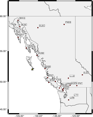
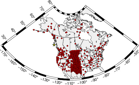
The focal mechanism was determined using broadband seismic waveforms. The location of the event (star) and the stations used for (red) the waveform inversion are shown in the next figure.
|
|
|
The program wvfgrd96 was used with good traces observed at short distance to determine the focal mechanism, depth and seismic moment. This technique requires a high quality signal and well determined velocity model for the Green's functions. To the extent that these are the quality data, this type of mechanism should be preferred over the radiation pattern technique which requires the separate step of defining the pressure and tension quadrants and the correct strike.
The observed and predicted traces are filtered using the following gsac commands:
hp c 0.01 n 3
lp c 0.025 n 3
The results of this grid search are as follow:
           DEPTH  STK   DIP  RAKE   MW    FIT
WVFGRD96    0.5    90    75    20   6.16 0.4409
WVFGRD96    1.0    90    70    15   6.18 0.4583
WVFGRD96    2.0    90    70    15   6.21 0.5029
WVFGRD96    3.0    90    70    15   6.23 0.5260
WVFGRD96    4.0    90    70    15   6.25 0.5423
WVFGRD96    5.0    90    70    15   6.26 0.5541
WVFGRD96    6.0    85    75     0   6.26 0.5658
WVFGRD96    7.0    85    75     0   6.28 0.5763
WVFGRD96    8.0    85    75     0   6.29 0.5851
WVFGRD96    9.0    85    75     0   6.30 0.5909
WVFGRD96   10.0    85    75     0   6.31 0.5940
WVFGRD96   11.0    85    80     0   6.31 0.5949
WVFGRD96   12.0    85    80     0   6.32 0.5947
WVFGRD96   13.0    85    80     0   6.33 0.5928
WVFGRD96   14.0    85    80     0   6.33 0.5899
WVFGRD96   15.0    85    80    -5   6.34 0.5860
WVFGRD96   16.0    85    80    -5   6.34 0.5819
WVFGRD96   17.0    85    80   -10   6.35 0.5776
WVFGRD96   18.0    85    80   -10   6.35 0.5731
WVFGRD96   19.0    85    80   -10   6.36 0.5684
WVFGRD96   20.0   265    90     0   6.36 0.5546
WVFGRD96   21.0   270    75    25   6.37 0.5539
WVFGRD96   22.0   270    75    25   6.38 0.5540
WVFGRD96   23.0   270    75    25   6.38 0.5544
WVFGRD96   24.0   270    75    25   6.39 0.5545
WVFGRD96   25.0   270    75    25   6.39 0.5546
WVFGRD96   26.0   270    80    25   6.39 0.5552
WVFGRD96   27.0   270    80    25   6.40 0.5553
WVFGRD96   28.0   270    80    25   6.40 0.5554
WVFGRD96   29.0   270    80    25   6.41 0.5556
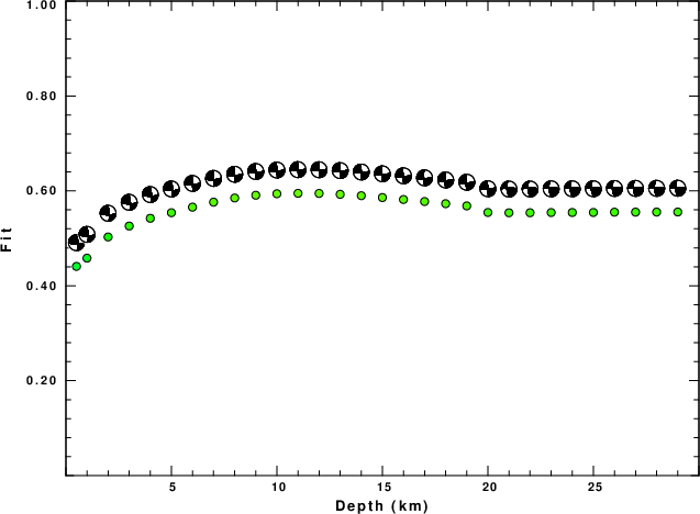
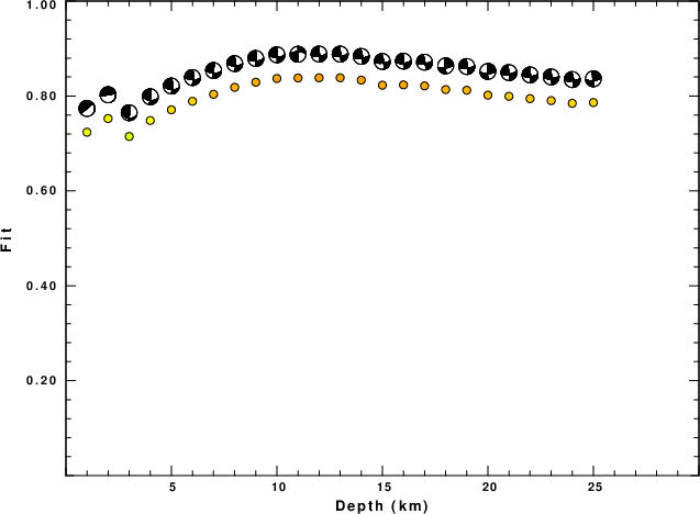
The best solution is
WVFGRD96 11.0 85 80 0 6.31 0.5949
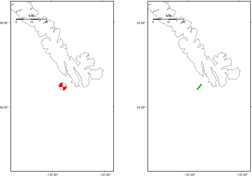
The mechanism corresponding to the best fit is
|
|
|
The best fit as a function of depth is given in the following figure:
|
|
|
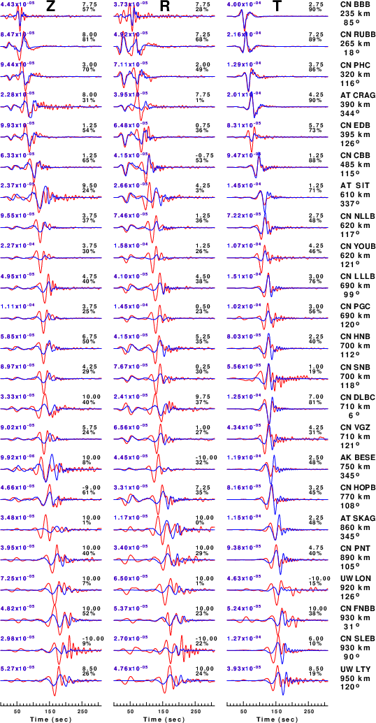
The comparison of the observed and predicted waveforms is given in the next figure. The red traces are the observed and the blue are the predicted. Each observed-predicted component is plotted to the same scale and peak amplitudes are indicated by the numbers to the left of each trace. A pair of numbers is given in black at the right of each predicted traces. The upper number it the time shift required for maximum correlation between the observed and predicted traces. This time shift is required because the synthetics are not computed at exactly the same distance as the observed, the velocity model used in the predictions may not be perfect and the epicentral parameters may be be off. A positive time shift indicates that the prediction is too fast and should be delayed to match the observed trace (shift to the right in this figure). A negative value indicates that the prediction is too slow. The lower number gives the percentage of variance reduction to characterize the individual goodness of fit (100% indicates a perfect fit).
The bandpass filter used in the processing and for the display was
hp c 0.01 n 3
lp c 0.025 n 3
|
| Figure 3. Waveform comparison for selected depth. Red: observed; Blue - predicted. The time shift with respect to the model prediction is indicated. The percent of fit is also indicated. The time scale is relative to the first trace sample. |
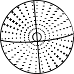
|
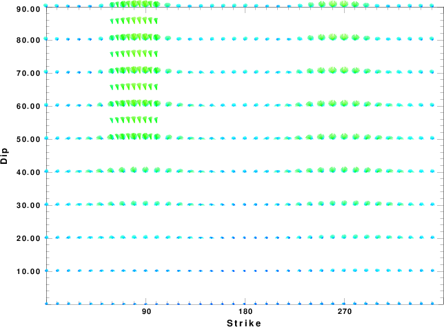
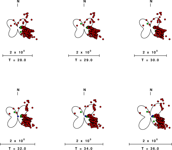
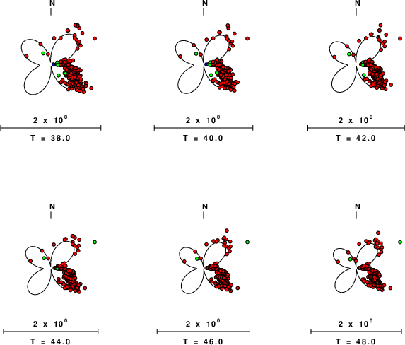
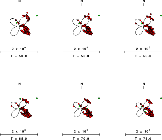
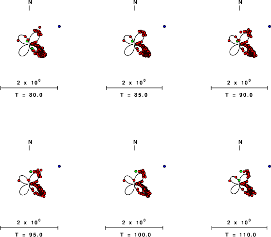
| Focal mechanism sensitivity at the preferred depth. The red color indicates a very good fit to the waveforms. Each solution is plotted as a vector at a given value of strike and dip with the angle of the vector representing the rake angle, measured, with respect to the upward vertical (N) in the figure. |
A check on the assumed source location is possible by looking at the time shifts between the observed and predicted traces. The time shifts for waveform matching arise for several reasons:
Time_shift = A + B cos Azimuth + C Sin Azimuth
The time shifts for this inversion lead to the next figure:
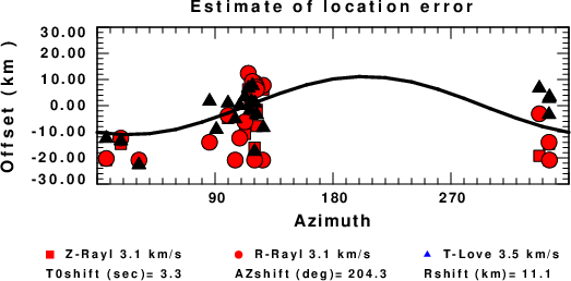
The derived shift in origin time and epicentral coordinates are given at the bottom of the figure.
The following figure shows the stations used in the grid search for the best focal mechanism to fit the surface-wave spectral amplitudes of the Love and Rayleigh waves.
|
|
|
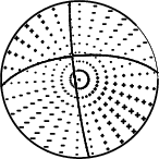
The surface-wave determined focal mechanism is shown here.
  NODAL PLANES


  STK=     172.87
  DIP=      85.47
 RAKE=     154.92

             OR

  STK=     264.98
  DIP=      65.00
 RAKE=       5.00


DEPTH = 12.0 km

Mw = 6.48
Best Fit 0.8384 - P-T axis plot gives solutions with FIT greater than FIT90
 |
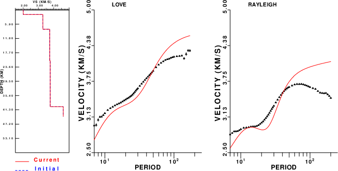
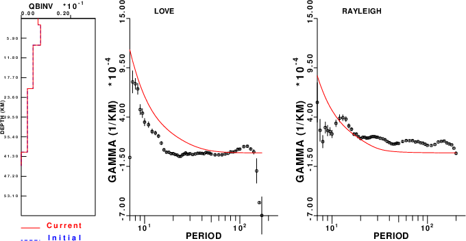
Surface wave analysis was performed using codes from Computer Programs in Seismology, specifically the multiple filter analysis program do_mft and the surface-wave radiation pattern search program srfgrd96.
Digital data were collected, instrument response removed and traces converted
to Z, R an T components. Multiple filter analysis was applied to the Z and T traces to obtain the Rayleigh- and Love-wave spectral amplitudes, respectively.
These were input to the search program which examined all depths between 1 and 25 km
and all possible mechanisms.
|
|
|
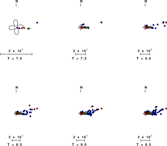
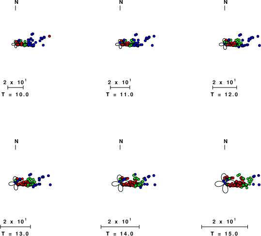
|
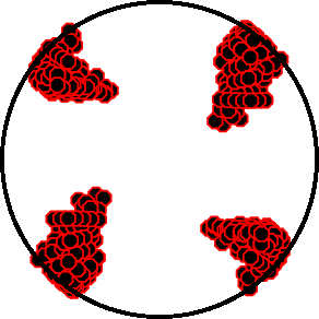
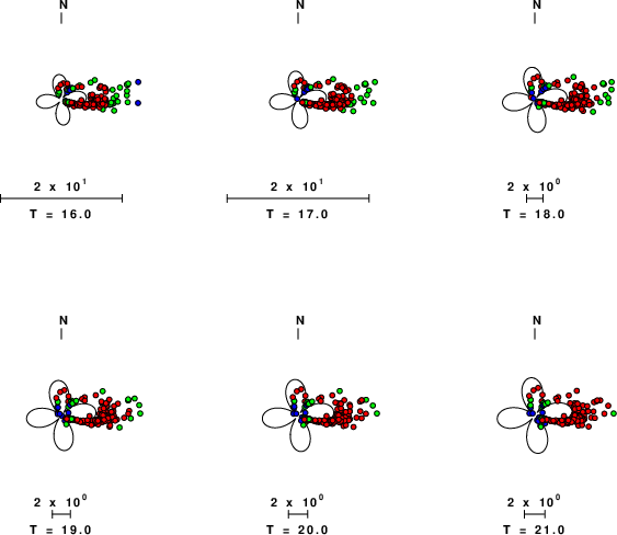
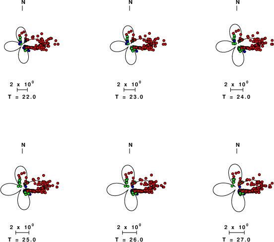
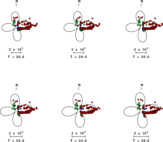
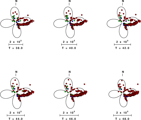
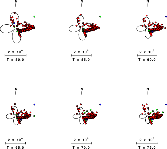
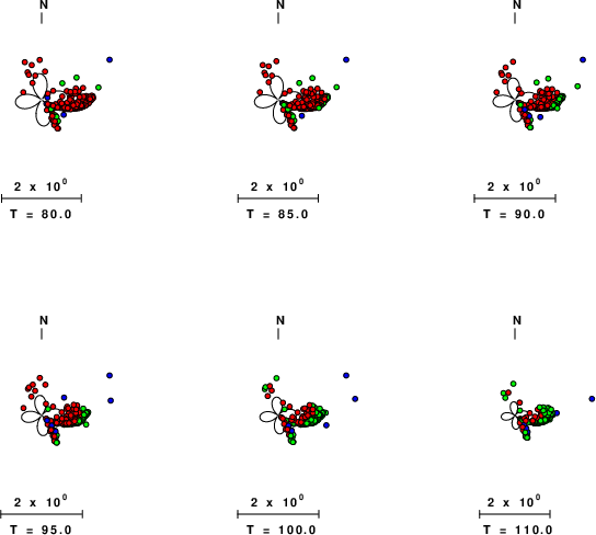
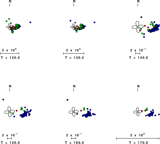
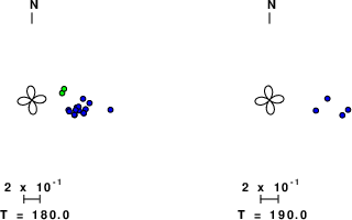
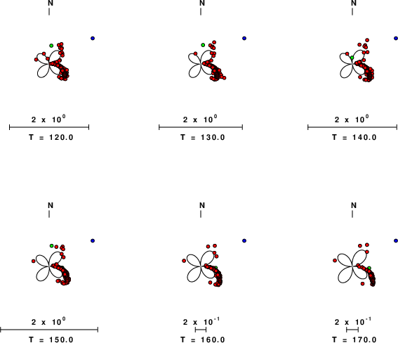
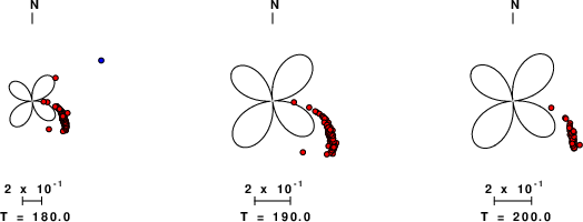
| Pressure-tension axis trends. Since the surface-wave spectra search does not distinguish between P and T axes and since there is a 180 ambiguity in strike, all possible P and T axes are plotted. First motion data and waveforms will be used to select the preferred mechanism. The purpose of this plot is to provide an idea of the possible range of solutions. The P and T-axes for all mechanisms with goodness of fit greater than 0.9 FITMAX (above) are plotted here. |
|
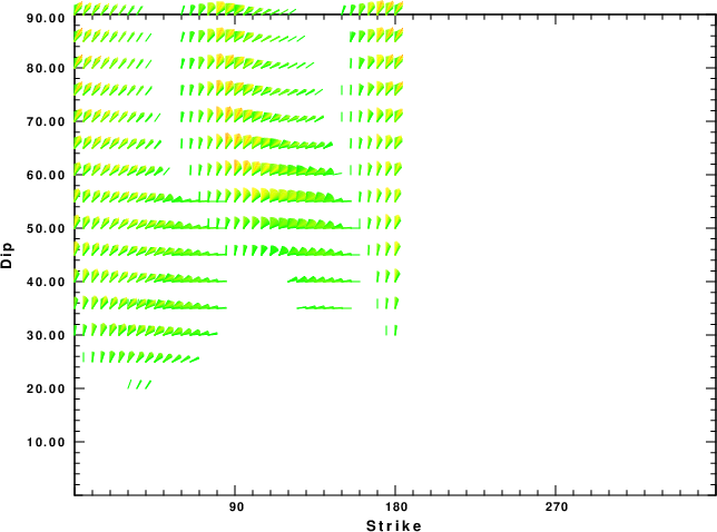
| Focal mechanism sensitivity at the preferred depth. The red color indicates a very good fit to the Love and Rayleigh wave radiation patterns. Each solution is plotted as a vector at a given value of strike and dip with the angle of the vector representing the rake angle, measured, with respect to the upward vertical (N) in the figure. Because of the symmetry of the spectral amplitude rediation patterns, only strikes from 0-180 degrees are sampled. |
|
|
The WUS.model used for the waveform synthetic seismograms and for the surface wave eigenfunctions and dispersion is as follows (The format is in the model96 format of Computer Programs in Seismology).
MODEL.01
Model after     8 iterations
ISOTROPIC
KGS
FLAT EARTH
1-D
CONSTANT VELOCITY
LINE08
LINE09
LINE10
LINE11
      H(KM)   VP(KM/S)   VS(KM/S) RHO(GM/CC)         QP         QS       ETAP       ETAS      FREFP      FREFS
     1.9000     3.4065     2.0089     2.2150  0.302E-02  0.679E-02   0.00       0.00       1.00       1.00
     6.1000     5.5445     3.2953     2.6089  0.349E-02  0.784E-02   0.00       0.00       1.00       1.00
    13.0000     6.2708     3.7396     2.7812  0.212E-02  0.476E-02   0.00       0.00       1.00       1.00
    19.0000     6.4075     3.7680     2.8223  0.111E-02  0.249E-02   0.00       0.00       1.00       1.00
     0.0000     7.9000     4.6200     3.2760  0.164E-10  0.370E-10   0.00       0.00       1.00       1.00