Location

Location ANSS

The ANSS event ID is nn00294871 and the event page is at https://earthquake.usgs.gov/earthquakes/eventpage/nn00294871/executive.

2009/10/09 22:13:54 36.042 -114.558 12.0 3.3 Arizona

Focal Mechanism

USGS/SLU Moment Tensor Solution ENS 2009/10/09 22:13:54:0 36.04 -114.56 12.0 3.3 Arizona Stations used: BK.CMB CI.GLA CI.GSC CI.ISA CI.LDF II.PFO IU.TUC TA.R11A TA.U20A TA.V20A TA.W18A TA.Y12C US.DUG Filtering commands used: hp c 0.02 n 3 lp c 0.10 n 3 br c 0.12 0.25 n 4 p 2 Best Fitting Double Couple Mo = 1.95e+21 dyne-cm Mw = 3.46 Z = 9 km Plane Strike Dip Rake NP1 105 85 20 NP2 13 70 175 Principal Axes: Axis Value Plunge Azimuth T 1.95e+21 18 331 N 0.00e+00 69 118 P -1.95e+21 10 237 Moment Tensor: (dyne-cm) Component Value Mxx 8.05e+20 Mxy -1.61e+21 Mxz 6.76e+20 Myy -9.20e+20 Myz 1.57e+19 Mzz 1.16e+20 ############-- # #############----- #### T #############-------- ##### #############--------- #######################----------- ########################------------ #########################------------- ##########################-------------- --########################-------------- -------####################--------------- -------------#############---------------- --------------------######---------------- --------------------------#--------------- ------------------------###########----- -----------------------################# -- -----------------################ - P ----------------################ ---------------################ ---------------############### -------------############### ---------############# ---########### Global CMT Convention Moment Tensor: R T P 1.16e+20 6.76e+20 -1.57e+19 6.76e+20 8.05e+20 1.61e+21 -1.57e+19 1.61e+21 -9.20e+20 Details of the solution is found at http://www.eas.slu.edu/eqc/eqc_mt/MECH.NA/20091009221354/index.html

Preferred Solution

      STK = 105
      DIP = 85
     RAKE = 20
       MW = 3.46
       HS = 9.0

The NDK file is 20091009221354.ndk The waveform inversion is preferred.

Moment Tensor Comparison

The following compares this source inversion to those provided by others. The purpose is to look for major differences and also to note slight differences that might be inherent to the processing procedure. For completeness the USGS/SLU solution is repeated from above.

SLU	UNR
USGS/SLU Moment Tensor Solution ENS 2009/10/09 22:13:54:0 36.04 -114.56 12.0 3.3 Arizona Stations used: BK.CMB CI.GLA CI.GSC CI.ISA CI.LDF II.PFO IU.TUC TA.R11A TA.U20A TA.V20A TA.W18A TA.Y12C US.DUG Filtering commands used: hp c 0.02 n 3 lp c 0.10 n 3 br c 0.12 0.25 n 4 p 2 Best Fitting Double Couple Mo = 1.95e+21 dyne-cm Mw = 3.46 Z = 9 km Plane Strike Dip Rake NP1 105 85 20 NP2 13 70 175 Principal Axes: Axis Value Plunge Azimuth T 1.95e+21 18 331 N 0.00e+00 69 118 P -1.95e+21 10 237 Moment Tensor: (dyne-cm) Component Value Mxx 8.05e+20 Mxy -1.61e+21 Mxz 6.76e+20 Myy -9.20e+20 Myz 1.57e+19 Mzz 1.16e+20 ############-- # #############----- #### T #############-------- ##### #############--------- #######################----------- ########################------------ #########################------------- ##########################-------------- --########################-------------- -------####################--------------- -------------#############---------------- --------------------######---------------- --------------------------#--------------- ------------------------###########----- -----------------------################# -- -----------------################ - P ----------------################ ---------------################ ---------------############### -------------############### ---------############# ---########### Global CMT Convention Moment Tensor: R T P 1.16e+20 6.76e+20 -1.57e+19 6.76e+20 8.05e+20 1.61e+21 -1.57e+19 1.61e+21 -9.20e+20 Details of the solution is found at http://www.eas.slu.edu/eqc/eqc_mt/MECH.NA/20091009221354/index.html	University of Nevada Reno Moment Tenor Solution Locl Magnitude 3.9 - local magnitude (ML) Moment Magnitude 3.49 - (Mw) Event Location Google Map 39.963 -114.546 Friday, October 9, 2009 at 3:13:54 PM (PDT) Friday, October 9, 2009 at 22:13:54.18 (UTC) 31 km from Boulder City, NV (19 miles) Azimuth E (85 degrees) 61 km from Las Vegas, NV (41 miles) Azimuth ESE (113 degrees) Event ID: 294871 Map: Event Station Geometry	Best Fit Solution Event ID: 294871 Date: 2009/10/09,22:13:54 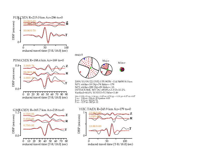Waveform Fits	Seismic Moment Tensor Solution 2009/10/09 (282) 22:13:52.00 35.9628 -114.5455 684215 Depth = 8.0 (km) Mw = 3.49 Mo = 2.12x10^21 (dyne x cm) Percent Double Couple = 90 % Percent CLVD = 10 % no ISO calculated Epsilon=0.05 Percent Variance Reduction = 60.01 % Total Fit = 5.34 Major Double Couple strike dip rake Nodal Plane 1: 18 74 -178 Nodal Plane 2: 288 89 -16 DEVIATORIC MOMENT TENSOR Moment Tensor Elements: Spherical Coordinates Mrr= 0.07 Mtt= 1.14 Mff= -1.21 Mrt= 0.53 Mrf= -0.27 Mtf= 1.65 EXP=21 Moment Tensor Elements: Cartesian Coordinates 1.14 -1.65 0.53 -1.65 -1.21 0.27 0.53 0.27 0.07 Eigenvalues: T-axis eigenvalue= 2.06 N-axis eigenvalue= 0.11 P-axis eigenvalue= -2.17 Eigenvalues and eigenvectors of the Major Double Couple: T-axis ev= 2.06 trend=334 plunge=10 N-axis ev= 0.00 trend=102 plunge=74 P-axis ev=-2.06 trend=242 plunge=12 Maximum Azmuithal Gap=243 Distance to Nearest Station=165.7 (km) Number of Stations (D=Displacement/V=Velocity) Used=4 (defining only) GMR.CI.D PDM.CI.D FUR.CI.D Y12C.TA.D ################- T ##################----- # ##################------- ########################--------- #########################---------- ##########################----------- -###########################------------- ############################------------- -###########################--------------- ------######################--------------- -----------################---------------- -----------------##########---------------- ----------------------#######-------------- ------------------------##########--------- ------------------------###############---- -----------------------#################### --------------------#################### P -------------------##################### ------------------##################### ----------------#################### -------------#################### ----------################### ------################### -################# # All Stations defining and nondefining: Station.Net Def Distance Azi Bazi lo-f hi-f vmodel (km) (deg) (deg) (Hz) (Hz) GMR.CI (D) Y 165.7 218 37 0.020 0.080 GMR.CI.wus.glib PDM.CI (D) Y 188.4 169 349 0.020 0.080 PDM.CI.wus.glib FUR.CI (D) Y 215.0 286 105 0.020 0.080 FUR.CI.wus.glib Y12C.TA (D) Y 245.9 179 359 0.020 0.080 Y12C.TA.wus.glib (V)-velocity (D)-Displacement Author: ken (Gene Inchinose MTINV Moment Tensor Solution Package) Date: 2009/10/10 03:35:47 mtinv Version 2.1_DEVEL OCT2008		Velocity Model: Western US Ritsema and Lay 1995 JGR. Z P QP S QS rho 4.00 4.52 500.00 2.61 250.00 2.39 28.00 6.21 500.00 3.59 250.00 2.76 20.00 7.73 1000.00 4.34 500.00 3.22 700.00 7.64 1000.00 4.29 500.00 3.19

Magnitudes

Given the availability of digital waveforms for determination of the moment tensor, this section documents the added processing leading to mLg, if appropriate to the region, and M_L by application of the respective IASPEI formulae. As a research study, the linear distance term of the IASPEI formula for M_L is adjusted to remove a linear distance trend in residuals to give a regionally defined M_L. The defined M_L uses horizontal component recordings, but the same procedure is applied to the vertical components since there may be some interest in vertical component ground motions. Residual plots versus distance may indicate interesting features of ground motion scaling in some distance ranges. A residual plot of the regionalized magnitude is given as a function of distance and azimuth, since data sets may transcend different wave propagation provinces.

ML Magnitude

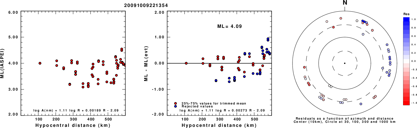
Left: ML computed using the IASPEI formula for Horizontal components. Center: ML residuals computed using a modified IASPEI formula that accounts for path specific attenuation; the values used for the trimmed mean are indicated. The ML relation used for each figure is given at the bottom of each plot. Right: Residuals from new relation as a function of distance and azimuth.

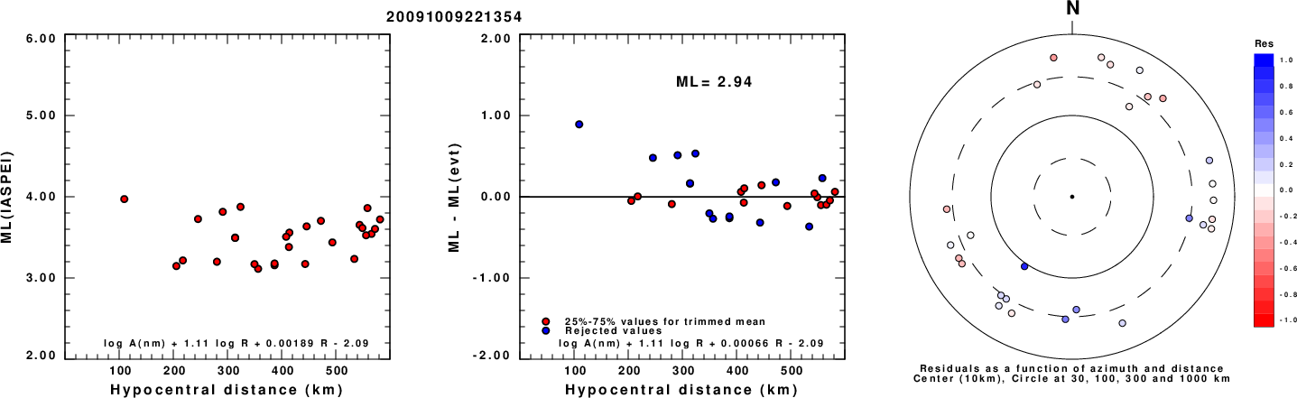
Left: ML computed using the IASPEI formula for Vertical components (research). Center: ML residuals computed using a modified IASPEI formula that accounts for path specific attenuation; the values used for the trimmed mean are indicated. The ML relation used for each figure is given at the bottom of each plot. Right: Residuals from new relation as a function of distance and azimuth.

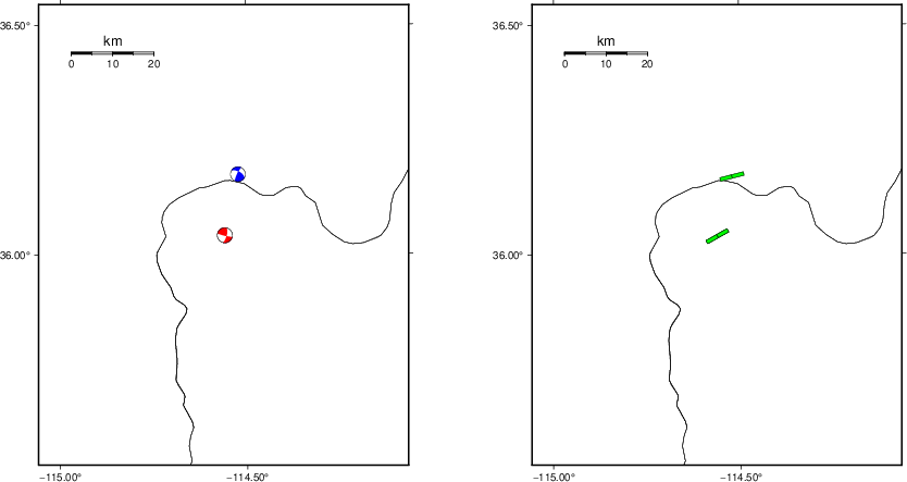
Context

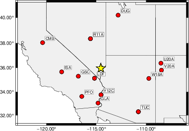
Waveform Inversion using wvfgrd96

The focal mechanism was determined using broadband seismic waveforms. The location of the event (star) and the stations used for (red) the waveform inversion are shown in the next figure.

Location of broadband stations used for waveform inversion

The program wvfgrd96 was used with good traces observed at short distance to determine the focal mechanism, depth and seismic moment. This technique requires a high quality signal and well determined velocity model for the Green's functions. To the extent that these are the quality data, this type of mechanism should be preferred over the radiation pattern technique which requires the separate step of defining the pressure and tension quadrants and the correct strike.

The observed and predicted traces are filtered using the following gsac commands:

hp c 0.02 n 3
lp c 0.10 n 3
br c 0.12 0.25 n 4 p 2

           DEPTH  STK   DIP  RAKE   MW    FIT
WVFGRD96    0.5   275    70   -10   3.09 0.2061
WVFGRD96    1.0    95    90     0   3.13 0.2319
WVFGRD96    2.0   100    80   -10   3.26 0.3490
WVFGRD96    3.0   105    90     5   3.30 0.3919
WVFGRD96    4.0   285    90   -10   3.33 0.4148
WVFGRD96    5.0   285    90   -15   3.37 0.4291
WVFGRD96    6.0   105    85    20   3.40 0.4407
WVFGRD96    7.0   105    85    20   3.42 0.4473
WVFGRD96    8.0   105    85    20   3.44 0.4520
WVFGRD96    9.0   105    85    20   3.46 0.4531
WVFGRD96   10.0   105    85    20   3.47 0.4530
WVFGRD96   11.0   105    85    20   3.49 0.4517
WVFGRD96   12.0   105    85    15   3.50 0.4498
WVFGRD96   13.0   105    90    15   3.51 0.4487
WVFGRD96   14.0   105    90    15   3.52 0.4468
WVFGRD96   15.0   105    90    15   3.53 0.4445
WVFGRD96   16.0   105    90    15   3.54 0.4414
WVFGRD96   17.0   285    90   -15   3.55 0.4374
WVFGRD96   18.0   285    85   -15   3.56 0.4335
WVFGRD96   19.0   285    85   -15   3.57 0.4298
WVFGRD96   20.0   285    70    10   3.58 0.4249
WVFGRD96   21.0   285    75    10   3.59 0.4212
WVFGRD96   22.0   285    75    10   3.60 0.4165
WVFGRD96   23.0   285    75    10   3.60 0.4110
WVFGRD96   24.0   285    70    10   3.61 0.4050
WVFGRD96   25.0   285    70    10   3.62 0.3993
WVFGRD96   26.0   285    70    10   3.63 0.3924
WVFGRD96   27.0   285    70    10   3.63 0.3845
WVFGRD96   28.0   290    65    15   3.64 0.3770
WVFGRD96   29.0   285    70    15   3.65 0.3692

The best solution is

WVFGRD96    9.0   105    85    20   3.46 0.4531

The mechanism corresponding to the best fit is

Figure 1. Waveform inversion focal mechanism

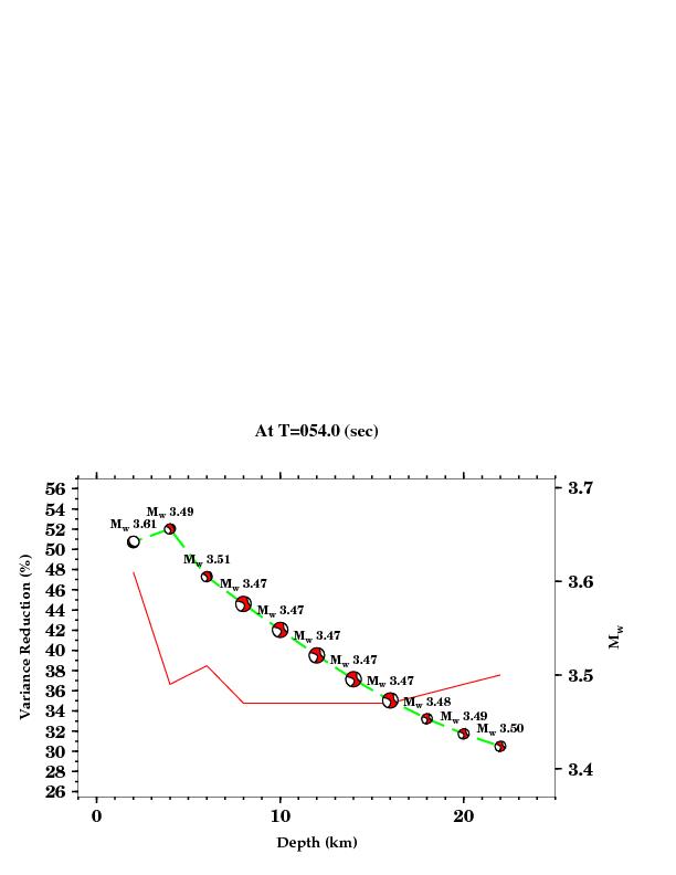
The best fit as a function of depth is given in the following figure:

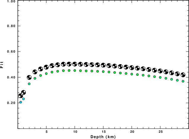
Figure 2. Depth sensitivity for waveform mechanism

The comparison of the observed and predicted waveforms is given in the next figure. The red traces are the observed and the blue are the predicted. Each observed-predicted component is plotted to the same scale and peak amplitudes are indicated by the numbers to the left of each trace. A pair of numbers is given in black at the right of each predicted traces. The upper number it the time shift required for maximum correlation between the observed and predicted traces. This time shift is required because the synthetics are not computed at exactly the same distance as the observed, the velocity model used in the predictions may not be perfect and the epicentral parameters may be be off. A positive time shift indicates that the prediction is too fast and should be delayed to match the observed trace (shift to the right in this figure). A negative value indicates that the prediction is too slow. The lower number gives the percentage of variance reduction to characterize the individual goodness of fit (100% indicates a perfect fit).

The bandpass filter used in the processing and for the display was

hp c 0.02 n 3
lp c 0.10 n 3
br c 0.12 0.25 n 4 p 2

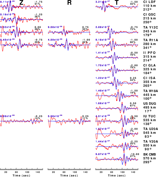
Figure 3. Waveform comparison for selected depth. Red: observed; Blue - predicted. The time shift with respect to the model prediction is indicated. The percent of fit is also indicated. The time scale is relative to the first trace sample.

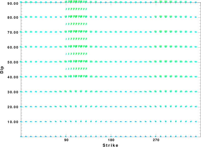
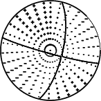
Focal mechanism sensitivity at the preferred depth. The red color indicates a very good fit to the waveforms. Each solution is plotted as a vector at a given value of strike and dip with the angle of the vector representing the rake angle, measured, with respect to the upward vertical (N) in the figure.

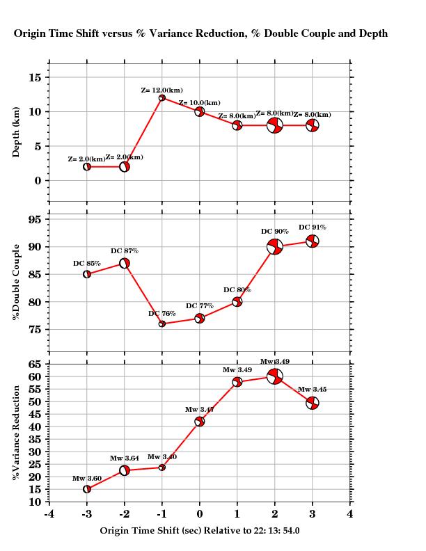
A check on the assumed source location is possible by looking at the time shifts between the observed and predicted traces. The time shifts for waveform matching arise for several reasons:

• The origin time and epicentral distance are incorrect
• The velocity model used for the inversion is incorrect
• The velocity model used to define the P-arrival time is not the same as the velocity model used for the waveform inversion (assuming that the initial trace alignment is based on the P arrival time)

 Time_shift = A + B cos Azimuth + C Sin Azimuth

The time shifts for this inversion lead to the next figure:

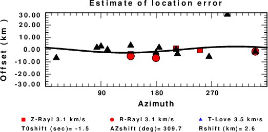
The derived shift in origin time and epicentral coordinates are given at the bottom of the figure.

Velocity Model

The WUS.model used for the waveform synthetic seismograms and for the surface wave eigenfunctions and dispersion is as follows (The format is in the model96 format of Computer Programs in Seismology).

MODEL.01
Model after     8 iterations
ISOTROPIC
KGS
FLAT EARTH
1-D
CONSTANT VELOCITY
LINE08
LINE09
LINE10
LINE11
      H(KM)   VP(KM/S)   VS(KM/S) RHO(GM/CC)         QP         QS       ETAP       ETAS      FREFP      FREFS
     1.9000     3.4065     2.0089     2.2150  0.302E-02  0.679E-02   0.00       0.00       1.00       1.00    
     6.1000     5.5445     3.2953     2.6089  0.349E-02  0.784E-02   0.00       0.00       1.00       1.00    
    13.0000     6.2708     3.7396     2.7812  0.212E-02  0.476E-02   0.00       0.00       1.00       1.00    
    19.0000     6.4075     3.7680     2.8223  0.111E-02  0.249E-02   0.00       0.00       1.00       1.00    
     0.0000     7.9000     4.6200     3.2760  0.164E-10  0.370E-10   0.00       0.00       1.00       1.00