Location
Location ANSS
The ANSS event ID is uw10762533 and the event page is at
https://earthquake.usgs.gov/earthquakes/eventpage/uw10762533/executive.
2009/02/26 09:52:47 42.541 -123.896 36.8 4.24 Oregon
Focal Mechanism
 USGS/SLU Moment Tensor Solution
 ENS  2009/02/26 09:52:47:0  42.54 -123.90  36.8 4.2 Oregon

 Stations used:
   BK.HUMO BK.WDC NC.KRMB UO.PIN US.BMO UW.LCCR UW.TREE
   UW.UMAT UW.YACT

 Filtering commands used:
   hp c 0.02 n 3
   lp c 0.06 n 3
   br c 0.12 0.25 n 4 p 2

 Best Fitting Double Couple
  Mo = 2.43e+22 dyne-cm
  Mw = 4.19
  Z  = 43 km
  Plane   Strike  Dip  Rake
   NP1      325    70   -75
   NP2      107    25   -125
  Principal Axes:
   Axis    Value   Plunge  Azimuth
    T   2.43e+22     24      43
    N   0.00e+00     14     140
    P  -2.43e+22     62     258

 Moment Tensor: (dyne-cm)
    Component   Value
       Mxx     1.05e+22
       Mxy     9.10e+21
       Mxz     8.54e+21
       Myy     4.56e+21
       Myz     1.59e+22
       Mzz    -1.51e+22


                     ##############
                 ######################
              -----#######################
             ---------################   ##
           -------------############## T ####
          ----------------############   #####
         -------------------###################
        ---------------------###################
        -----------------------#################
       #------------------------#################
       #------------   -----------###############
       ##----------- P ------------##############
       ###----------   -------------#############
        ##---------------------------###########
        ####-------------------------###########
         ####-------------------------########-
          #####------------------------######-
           ######----------------------####--
             #######-----------------------
              ############--------######--
                 ######################
                     ##############


 Global CMT Convention Moment Tensor:
      R          T          P
 -1.51e+22   8.54e+21  -1.59e+22
  8.54e+21   1.05e+22  -9.10e+21
 -1.59e+22  -9.10e+21   4.56e+21


Details of the solution is found at

http://www.eas.slu.edu/eqc/eqc_mt/MECH.NA/20090226095247/index.html
|
Preferred Solution
The preferred solution from an analysis of the surface-wave spectral amplitude radiation pattern, waveform inversion or first motion observations is
      STK = 325
      DIP = 70
     RAKE = -75
       MW = 4.19
       HS = 43.0
The NDK file is 20090226095247.ndk
The waveform inversion is preferred.
Moment Tensor Comparison
The following compares this source inversion to those provided by others. The purpose is to look for major differences and also to note slight differences that might be inherent to the processing procedure. For completeness the USGS/SLU solution is repeated from above.
| SLU |
PNSN |
 USGS/SLU Moment Tensor Solution
 ENS  2009/02/26 09:52:47:0  42.54 -123.90  36.8 4.2 Oregon

 Stations used:
   BK.HUMO BK.WDC NC.KRMB UO.PIN US.BMO UW.LCCR UW.TREE
   UW.UMAT UW.YACT

 Filtering commands used:
   hp c 0.02 n 3
   lp c 0.06 n 3
   br c 0.12 0.25 n 4 p 2

 Best Fitting Double Couple
  Mo = 2.43e+22 dyne-cm
  Mw = 4.19
  Z  = 43 km
  Plane   Strike  Dip  Rake
   NP1      325    70   -75
   NP2      107    25   -125
  Principal Axes:
   Axis    Value   Plunge  Azimuth
    T   2.43e+22     24      43
    N   0.00e+00     14     140
    P  -2.43e+22     62     258

 Moment Tensor: (dyne-cm)
    Component   Value
       Mxx     1.05e+22
       Mxy     9.10e+21
       Mxz     8.54e+21
       Myy     4.56e+21
       Myz     1.59e+22
       Mzz    -1.51e+22


                     ##############
                 ######################
              -----#######################
             ---------################   ##
           -------------############## T ####
          ----------------############   #####
         -------------------###################
        ---------------------###################
        -----------------------#################
       #------------------------#################
       #------------   -----------###############
       ##----------- P ------------##############
       ###----------   -------------#############
        ##---------------------------###########
        ####-------------------------###########
         ####-------------------------########-
          #####------------------------######-
           ######----------------------####--
             #######-----------------------
              ############--------######--
                 ######################
                     ##############


 Global CMT Convention Moment Tensor:
      R          T          P
 -1.51e+22   8.54e+21  -1.59e+22
  8.54e+21   1.05e+22  -9.10e+21
 -1.59e+22  -9.10e+21   4.56e+21


Details of the solution is found at

http://www.eas.slu.edu/eqc/eqc_mt/MECH.NA/20090226095247/index.html
|
Fault Plane Parameters for 09022609524k
Fault        Choice 1    Fault Choice 2
Strike(deg)    120.0       330.0
Dip(deg)        50.0        44.0
Rake(deg)     -110.3       -67.5
Fault Type    normal       normal


PNSN Notable Quake link for this earthquake
|
Magnitudes
Given the availability of digital waveforms for determination of the moment tensor, this section documents the added processing leading to mLg, if appropriate to the region, and ML by application of the respective IASPEI formulae. As a research study, the linear distance term of the IASPEI formula
for ML is adjusted to remove a linear distance trend in residuals to give a regionally defined ML. The defined ML uses horizontal component recordings, but the same procedure is applied to the vertical components since there may be some interest in vertical component ground motions. Residual plots versus distance may indicate interesting features of ground motion scaling in some distance ranges. A residual plot of the regionalized magnitude is given as a function of distance and azimuth, since data sets may transcend different wave propagation provinces.
ML Magnitude
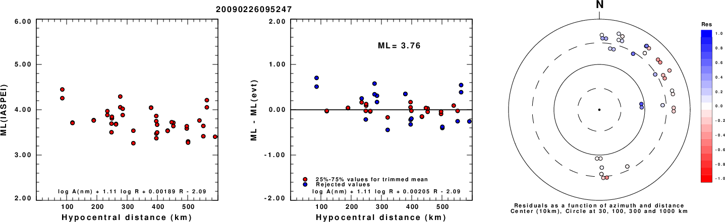
Left: ML computed using the IASPEI formula for Horizontal components. Center: ML residuals computed using a modified IASPEI formula that accounts for path specific attenuation; the values used for the trimmed mean are indicated. The ML relation used for each figure is given at the bottom of each plot.
Right: Residuals from new relation as a function of distance and azimuth.
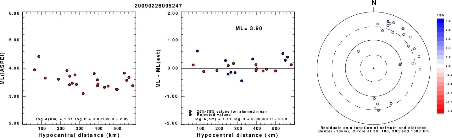
Left: ML computed using the IASPEI formula for Vertical components (research). Center: ML residuals computed using a modified IASPEI formula that accounts for path specific attenuation; the values used for the trimmed mean are indicated. The ML relation used for each figure is given at the bottom of each plot.
Right: Residuals from new relation as a function of distance and azimuth.
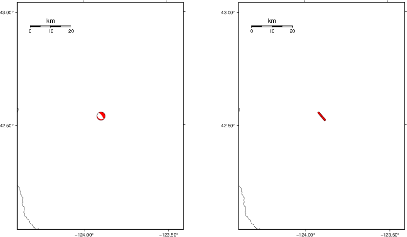
Context
The left panel of the next figure presents the focal mechanism for this earthquake (red) in the context of other nearby events (blue) in the SLU Moment Tensor Catalog. The right panel shows the inferred direction of maximum compressive stress and the type of faulting (green is strike-slip, red is normal, blue is thrust; oblique is shown by a combination of colors). Thus context plot is useful for assessing the appropriateness of the moment tensor of this event.
Waveform Inversion using wvfgrd96
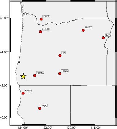
The focal mechanism was determined using broadband seismic waveforms. The location of the event (star) and the
stations used for (red) the waveform inversion are shown in the next figure.
|
|
Location of broadband stations used for waveform inversion
|
The program wvfgrd96 was used with good traces observed at short distance to determine the focal mechanism, depth and seismic moment. This technique requires a high quality signal and well determined velocity model for the Green's functions. To the extent that these are the quality data, this type of mechanism should be preferred over the radiation pattern technique which requires the separate step of defining the pressure and tension quadrants and the correct strike.
The observed and predicted traces are filtered using the following gsac commands:
hp c 0.02 n 3
lp c 0.06 n 3
br c 0.12 0.25 n 4 p 2
The results of this grid search are as follow:
           DEPTH  STK   DIP  RAKE   MW    FIT
WVFGRD96    0.5   320    75    15   3.60 0.2469
WVFGRD96    1.0   320    75    10   3.63 0.2604
WVFGRD96    2.0   320    75    10   3.71 0.2941
WVFGRD96    3.0   320    70    10   3.76 0.3052
WVFGRD96    4.0   320    70    10   3.80 0.3033
WVFGRD96    5.0   320    70    10   3.82 0.2917
WVFGRD96    6.0   315    65    -5   3.84 0.2788
WVFGRD96    7.0   315    60   -10   3.84 0.2687
WVFGRD96    8.0   155    75    55   3.84 0.2638
WVFGRD96    9.0   155    75    55   3.83 0.2626
WVFGRD96   10.0   160    75    55   3.81 0.2654
WVFGRD96   11.0   155    80    50   3.81 0.2697
WVFGRD96   12.0   160    80    55   3.80 0.2761
WVFGRD96   13.0   160    80    55   3.80 0.2832
WVFGRD96   14.0   160    80    55   3.80 0.2902
WVFGRD96   15.0   165    80    55   3.80 0.2975
WVFGRD96   16.0   160    85    55   3.80 0.3060
WVFGRD96   17.0   160    85    55   3.81 0.3142
WVFGRD96   18.0   330    85   -50   3.83 0.3228
WVFGRD96   19.0   330    80   -50   3.84 0.3330
WVFGRD96   20.0   330    80   -55   3.84 0.3439
WVFGRD96   21.0   325    75   -55   3.87 0.3543
WVFGRD96   22.0   325    75   -55   3.88 0.3670
WVFGRD96   23.0   325    70   -55   3.89 0.3807
WVFGRD96   24.0   325    70   -55   3.91 0.3940
WVFGRD96   25.0   325    70   -55   3.92 0.4066
WVFGRD96   26.0   325    70   -60   3.93 0.4188
WVFGRD96   27.0   325    70   -60   3.94 0.4306
WVFGRD96   28.0   325    70   -60   3.95 0.4416
WVFGRD96   29.0   325    70   -60   3.96 0.4516
WVFGRD96   30.0   325    70   -65   3.97 0.4606
WVFGRD96   31.0   325    70   -65   3.98 0.4689
WVFGRD96   32.0   325    65   -65   3.99 0.4764
WVFGRD96   33.0   325    65   -65   4.00 0.4835
WVFGRD96   34.0   325    65   -65   4.01 0.4892
WVFGRD96   35.0   325    65   -65   4.02 0.4942
WVFGRD96   36.0   325    65   -65   4.02 0.4985
WVFGRD96   37.0   325    65   -65   4.03 0.5018
WVFGRD96   38.0   325    65   -65   4.04 0.5050
WVFGRD96   39.0   320    60   -70   4.07 0.5082
WVFGRD96   40.0   325    70   -75   4.17 0.5040
WVFGRD96   41.0   325    70   -75   4.18 0.5068
WVFGRD96   42.0   325    70   -75   4.18 0.5084
WVFGRD96   43.0   325    70   -75   4.19 0.5089
WVFGRD96   44.0   320    65   -75   4.20 0.5088
WVFGRD96   45.0   320    65   -75   4.20 0.5083
WVFGRD96   46.0   320    65   -75   4.21 0.5068
WVFGRD96   47.0   320    65   -75   4.21 0.5048
WVFGRD96   48.0   325    65   -75   4.22 0.5021
WVFGRD96   49.0   320    65   -75   4.22 0.4986
WVFGRD96   50.0   325    65   -70   4.22 0.4948
WVFGRD96   51.0   320    65   -75   4.23 0.4903
WVFGRD96   52.0   320    65   -75   4.23 0.4850
WVFGRD96   53.0   325    65   -70   4.23 0.4798
WVFGRD96   54.0   325    65   -70   4.23 0.4742
WVFGRD96   55.0   325    65   -70   4.23 0.4679
WVFGRD96   56.0   325    65   -70   4.23 0.4617
WVFGRD96   57.0   325    65   -70   4.23 0.4549
WVFGRD96   58.0   325    65   -70   4.24 0.4481
WVFGRD96   59.0   325    65   -70   4.24 0.4417
WVFGRD96   60.0   325    65   -70   4.24 0.4348
The best solution is
WVFGRD96 43.0 325 70 -75 4.19 0.5089
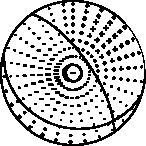
The mechanism corresponding to the best fit is
|
|
Figure 1. Waveform inversion focal mechanism
|
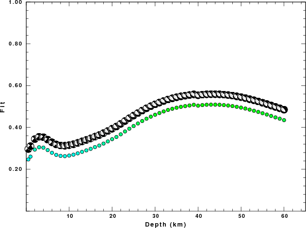
The best fit as a function of depth is given in the following figure:
|
|
Figure 2. Depth sensitivity for waveform mechanism
|
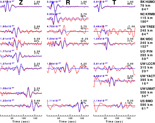
The comparison of the observed and predicted waveforms is given in the next figure. The red traces are the observed and the blue are the predicted.
Each observed-predicted component is plotted to the same scale and peak amplitudes are indicated by the numbers to the left of each trace. A pair of numbers is given in black at the right of each predicted traces. The upper number it the time shift required for maximum correlation between the observed and predicted traces. This time shift is required because the synthetics are not computed at exactly the same distance as the observed, the velocity model used in the predictions may not be perfect and the epicentral parameters may be be off.
A positive time shift indicates that the prediction is too fast and should be delayed to match the observed trace (shift to the right in this figure). A negative value indicates that the prediction is too slow. The lower number gives the percentage of variance reduction to characterize the individual goodness of fit (100% indicates a perfect fit).
The bandpass filter used in the processing and for the display was
hp c 0.02 n 3
lp c 0.06 n 3
br c 0.12 0.25 n 4 p 2
|
|
Figure 3. Waveform comparison for selected depth. Red: observed; Blue - predicted. The time shift with respect to the model prediction is indicated. The percent of fit is also indicated. The time scale is relative to the first trace sample.
|
|
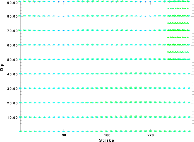
|
Focal mechanism sensitivity at the preferred depth. The red color indicates a very good fit to the waveforms.
Each solution is plotted as a vector at a given value of strike and dip with the angle of the vector representing the rake angle, measured, with respect to the upward vertical (N) in the figure.
|
A check on the assumed source location is possible by looking at the time shifts between the observed and predicted traces. The time shifts for waveform matching arise for several reasons:
- The origin time and epicentral distance are incorrect
- The velocity model used for the inversion is incorrect
- The velocity model used to define the P-arrival time is not the
same as the velocity model used for the waveform inversion
(assuming that the initial trace alignment is based on the
P arrival time)
Assuming only a mislocation, the time shifts are fit to a functional form:
Time_shift = A + B cos Azimuth + C Sin Azimuth
The time shifts for this inversion lead to the next figure:
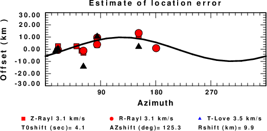
The derived shift in origin time and epicentral coordinates are given at the bottom of the figure.
Velocity Model
The WUS.model used for the waveform synthetic seismograms and for the surface wave eigenfunctions and dispersion is as follows
(The format is in the model96 format of Computer Programs in Seismology).
MODEL.01
Model after     8 iterations
ISOTROPIC
KGS
FLAT EARTH
1-D
CONSTANT VELOCITY
LINE08
LINE09
LINE10
LINE11
      H(KM)   VP(KM/S)   VS(KM/S) RHO(GM/CC)         QP         QS       ETAP       ETAS      FREFP      FREFS
     1.9000     3.4065     2.0089     2.2150  0.302E-02  0.679E-02   0.00       0.00       1.00       1.00
     6.1000     5.5445     3.2953     2.6089  0.349E-02  0.784E-02   0.00       0.00       1.00       1.00
    13.0000     6.2708     3.7396     2.7812  0.212E-02  0.476E-02   0.00       0.00       1.00       1.00
    19.0000     6.4075     3.7680     2.8223  0.111E-02  0.249E-02   0.00       0.00       1.00       1.00
     0.0000     7.9000     4.6200     3.2760  0.164E-10  0.370E-10   0.00       0.00       1.00       1.00
Last Changed Sun Apr 28 01:07:48 PM CDT 2024