Location
Location ANSS
The ANSS event ID is ci14408052 and the event page is at
https://earthquake.usgs.gov/earthquakes/eventpage/ci14408052/executive.
2008/12/06 04:18:42 34.813 -116.419 6.4 5.06 California
Focal Mechanism
 USGS/SLU Moment Tensor Solution
 ENS  2008/12/06 04:18:42:0  34.81 -116.42   6.4 5.1 California

 Stations used:
   AZ.LVA2 AZ.PFO AZ.RDM AZ.SOL CI.BAR CI.GLA CI.GSC CI.LDF
   CI.PASC

 Filtering commands used:
   hp c 0.02 n 3
   lp c 0.05 n 3

 Best Fitting Double Couple
  Mo = 4.12e+23 dyne-cm
  Mw = 5.01
  Z  = 9 km
  Plane   Strike  Dip  Rake
   NP1      165    90   -170
   NP2       75    80     0
  Principal Axes:
   Axis    Value   Plunge  Azimuth
    T   4.12e+23      7     300
    N   0.00e+00     80     165
    P  -4.12e+23      7      30

 Moment Tensor: (dyne-cm)
    Component   Value
       Mxx    -2.03e+23
       Mxy    -3.51e+23
       Mxz    -1.85e+22
       Myy     2.03e+23
       Myz    -6.91e+22
       Mzz     0.00e+00


                     ##------------
                 ######------------- P
              ##########------------   ---
             ###########-------------------
             ############--------------------
           T ############---------------------
         #   #############---------------------
        ##################----------------------
        ###################--------------------#
       ####################----------------######
       #####################-----------##########
       #####################------###############
       #####################-####################
        ###########----------###################
        ----------------------##################
         ---------------------#################
          ---------------------###############
           --------------------##############
             -------------------###########
              ------------------##########
                 ----------------######
                     ------------##


 Global CMT Convention Moment Tensor:
      R          T          P
  0.00e+00  -1.85e+22   6.91e+22
 -1.85e+22  -2.03e+23   3.51e+23
  6.91e+22   3.51e+23   2.03e+23


Details of the solution is found at

http://www.eas.slu.edu/eqc/eqc_mt/MECH.NA/20081206041842/index.html
|
Preferred Solution
The preferred solution from an analysis of the surface-wave spectral amplitude radiation pattern, waveform inversion or first motion observations is
      STK = 75
      DIP = 80
     RAKE = 0
       MW = 5.01
       HS = 9.0
The NDK file is 20081206041842.ndk
The waveform inversion is preferred.
Moment Tensor Comparison
The following compares this source inversion to those provided by others. The purpose is to look for major differences and also to note slight differences that might be inherent to the processing procedure. For completeness the USGS/SLU solution is repeated from above.
| SLU |
SCAL |
 USGS/SLU Moment Tensor Solution
 ENS  2008/12/06 04:18:42:0  34.81 -116.42   6.4 5.1 California

 Stations used:
   AZ.LVA2 AZ.PFO AZ.RDM AZ.SOL CI.BAR CI.GLA CI.GSC CI.LDF
   CI.PASC

 Filtering commands used:
   hp c 0.02 n 3
   lp c 0.05 n 3

 Best Fitting Double Couple
  Mo = 4.12e+23 dyne-cm
  Mw = 5.01
  Z  = 9 km
  Plane   Strike  Dip  Rake
   NP1      165    90   -170
   NP2       75    80     0
  Principal Axes:
   Axis    Value   Plunge  Azimuth
    T   4.12e+23      7     300
    N   0.00e+00     80     165
    P  -4.12e+23      7      30

 Moment Tensor: (dyne-cm)
    Component   Value
       Mxx    -2.03e+23
       Mxy    -3.51e+23
       Mxz    -1.85e+22
       Myy     2.03e+23
       Myz    -6.91e+22
       Mzz     0.00e+00


                     ##------------
                 ######------------- P
              ##########------------   ---
             ###########-------------------
             ############--------------------
           T ############---------------------
         #   #############---------------------
        ##################----------------------
        ###################--------------------#
       ####################----------------######
       #####################-----------##########
       #####################------###############
       #####################-####################
        ###########----------###################
        ----------------------##################
         ---------------------#################
          ---------------------###############
           --------------------##############
             -------------------###########
              ------------------##########
                 ----------------######
                     ------------##


 Global CMT Convention Moment Tensor:
      R          T          P
  0.00e+00  -1.85e+22   6.91e+22
 -1.85e+22  -2.03e+23   3.51e+23
  6.91e+22   3.51e+23   2.03e+23


Details of the solution is found at

http://www.eas.slu.edu/eqc/eqc_mt/MECH.NA/20081206041842/index.html
|
** SCSN Moment Tensor Solution Message **

REAL-TIME SOLUTION: OPERATOR REVIEWED
Reviewed On: 12/06/2008 4:34:40

Inversion Method: Complete Waveform
Number of Stations used: 6
Stations: CI.DSC CI.GMR CI.MCT CI.JVA CI.ADO CI.RRX

Real-Time Solution:
-------------------
Event ID    : 14408052
Magnitude   : 5.46
Depth (km)  : 6.0
Origin Time :  12/06/2008 04:18:42:550
Latitude    : 34.81
Longitude   : -116.42
Further Information at: http://pasadena.wr.usgs.gov/recenteqs/Quakes/ci14408052.htm

SCSN Moment Tensor Solution:
----------------------------
Moment Magnitude     : 5.06
Depth (km)           : 5
Variance Reduction(%): 94.07
Quality Factor       : A
   (A : Mw, MT good enough for distribution)
   (B : Mw only good enough for distribution)
   (C : Solution needs review before distribution)


Best Fitting Double Couple and CLVD Solution:
---------------------------------------------------

Moment Tensor: Scale = 10**21 Dyne-cm
    Component   Value
       Mxx      -251
       Mxy      -375
       Mxz      -75.6
       Myy      326
       Myz      -73.7
       Mzz      -74.8

Best Fitting Double Couple Solution:
--------------------------------------------------
 Moment Tensor: Scale = 10**23 Dyne-cm
    Component   Value
       Mxx     -2.749
       Mxy     -3.734
       Mxz     -0.959
       Myy      3.052
       Myz     -0.802
       Mzz     -0.304

 Principle Axes:
    Axis    Value   Plunge   Azimuth
      T     4.898       3      296
      N     0.000      75      193
      P    -4.898      15       27

 Best Fitting Double-Couple:
    Mo = 4.90E+23 Dyne-cm
    Plane   Strike   Rake   Dip
     NP1      162    -167    82
     NP2       70      -8    77

 Moment Magnitude = 5.06


                    -------
              ###----------------
           #######------------   ---
         #########------------ P -----
       ###########------------   -------
       ############----------------------
     T ############-----------------------
       ############------------------------
    ################---------------------##
   #################------------------######
   ##################--------------#########
   ###################---------#############
   ###################-----#################
   ###################-#####################
    ###########--------####################
    --------------------###################
     --------------------#################
      --------------------###############
       -------------------##############
         ------------------###########
           -----------------########
              ---------------####
                    -------

     Lower Hemisphere Equiangle Projection

=============  Station Information ==============

Name       Distance     Azimuth     VR      ZCore
-------------------------------------------------
CI.DSC       46.838     37.948   90.911      6.00
CI.GMR       69.614     92.106   94.957     10.00
CI.MCT       73.500    151.611   94.631     10.00
CI.JVA       52.301    199.807   95.550      7.00
CI.ADO       97.276    253.073   93.975     14.00
CI.RRX       53.256    277.985   94.482      8.00
|
|
Magnitudes
Given the availability of digital waveforms for determination of the moment tensor, this section documents the added processing leading to mLg, if appropriate to the region, and ML by application of the respective IASPEI formulae. As a research study, the linear distance term of the IASPEI formula
for ML is adjusted to remove a linear distance trend in residuals to give a regionally defined ML. The defined ML uses horizontal component recordings, but the same procedure is applied to the vertical components since there may be some interest in vertical component ground motions. Residual plots versus distance may indicate interesting features of ground motion scaling in some distance ranges. A residual plot of the regionalized magnitude is given as a function of distance and azimuth, since data sets may transcend different wave propagation provinces.
ML Magnitude
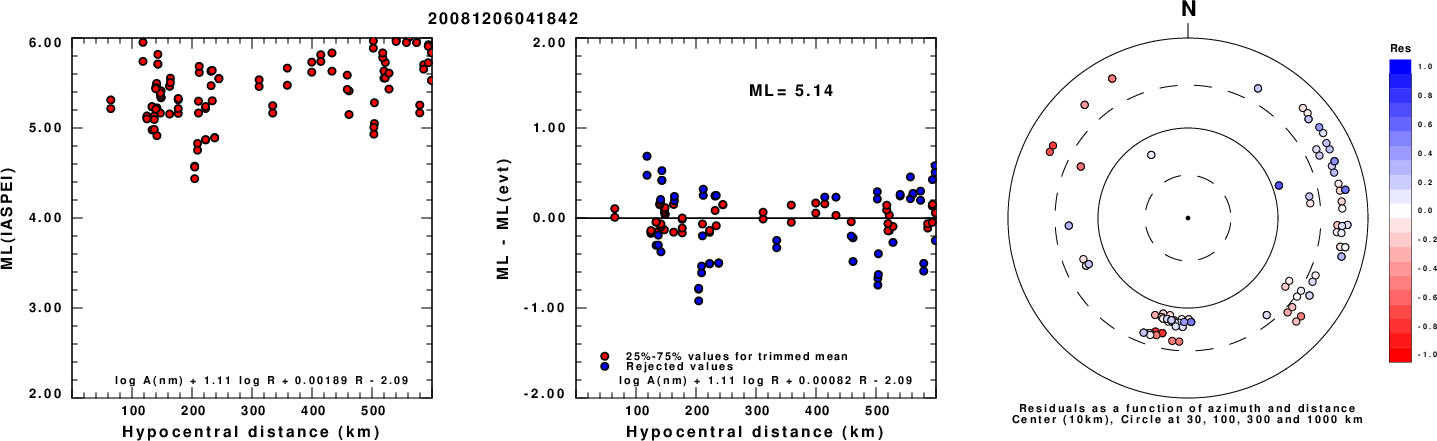
Left: ML computed using the IASPEI formula for Horizontal components. Center: ML residuals computed using a modified IASPEI formula that accounts for path specific attenuation; the values used for the trimmed mean are indicated. The ML relation used for each figure is given at the bottom of each plot.
Right: Residuals from new relation as a function of distance and azimuth.
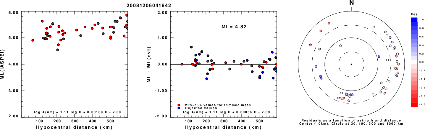
Left: ML computed using the IASPEI formula for Vertical components (research). Center: ML residuals computed using a modified IASPEI formula that accounts for path specific attenuation; the values used for the trimmed mean are indicated. The ML relation used for each figure is given at the bottom of each plot.
Right: Residuals from new relation as a function of distance and azimuth.
Context
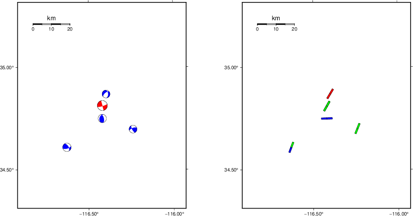
The left panel of the next figure presents the focal mechanism for this earthquake (red) in the context of other nearby events (blue) in the SLU Moment Tensor Catalog. The right panel shows the inferred direction of maximum compressive stress and the type of faulting (green is strike-slip, red is normal, blue is thrust; oblique is shown by a combination of colors). Thus context plot is useful for assessing the appropriateness of the moment tensor of this event.
Waveform Inversion using wvfgrd96
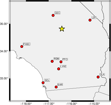
The focal mechanism was determined using broadband seismic waveforms. The location of the event (star) and the
stations used for (red) the waveform inversion are shown in the next figure.
|
|
Location of broadband stations used for waveform inversion
|
The program wvfgrd96 was used with good traces observed at short distance to determine the focal mechanism, depth and seismic moment. This technique requires a high quality signal and well determined velocity model for the Green's functions. To the extent that these are the quality data, this type of mechanism should be preferred over the radiation pattern technique which requires the separate step of defining the pressure and tension quadrants and the correct strike.
The observed and predicted traces are filtered using the following gsac commands:
hp c 0.02 n 3
lp c 0.05 n 3
The results of this grid search are as follow:
           DEPTH  STK   DIP  RAKE   MW    FIT
WVFGRD96    0.5   250    65   -20   4.73 0.4438
WVFGRD96    1.0    75    80   -15   4.74 0.4796
WVFGRD96    2.0    70    70   -25   4.86 0.6214
WVFGRD96    3.0    70    70   -20   4.89 0.6810
WVFGRD96    4.0    75    80    -5   4.90 0.7244
WVFGRD96    5.0    75    80    -5   4.93 0.7586
WVFGRD96    6.0    75    80    -5   4.95 0.7834
WVFGRD96    7.0    75    80     0   4.97 0.8030
WVFGRD96    8.0    75    80     0   5.00 0.8183
WVFGRD96    9.0    75    80     0   5.01 0.8224
WVFGRD96   10.0    75    80     0   5.02 0.8205
WVFGRD96   11.0    75    80     0   5.03 0.8141
WVFGRD96   12.0    75    80     0   5.04 0.8043
WVFGRD96   13.0    75    80     0   5.05 0.7929
WVFGRD96   14.0    75    80     5   5.06 0.7810
WVFGRD96   15.0    75    80     5   5.07 0.7702
WVFGRD96   16.0    75    80     5   5.08 0.7596
WVFGRD96   17.0    75    80     5   5.08 0.7488
WVFGRD96   18.0    75    80     5   5.09 0.7378
WVFGRD96   19.0    75    80     5   5.09 0.7264
The best solution is
WVFGRD96 9.0 75 80 0 5.01 0.8224
The mechanism corresponding to the best fit is
|
|
Figure 1. Waveform inversion focal mechanism
|
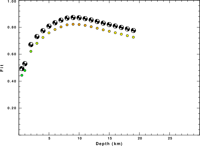
The best fit as a function of depth is given in the following figure:
|
|
Figure 2. Depth sensitivity for waveform mechanism
|
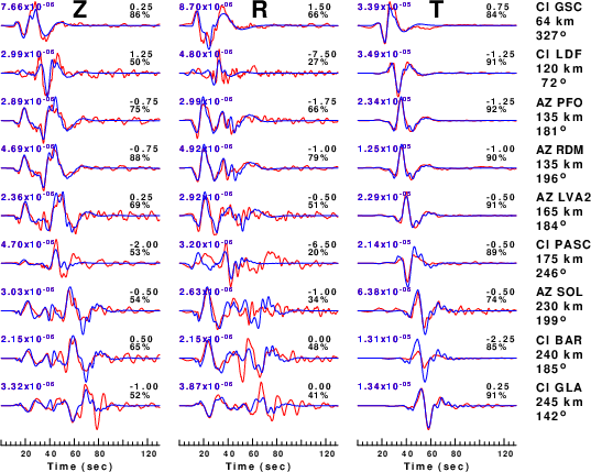
The comparison of the observed and predicted waveforms is given in the next figure. The red traces are the observed and the blue are the predicted.
Each observed-predicted component is plotted to the same scale and peak amplitudes are indicated by the numbers to the left of each trace. A pair of numbers is given in black at the right of each predicted traces. The upper number it the time shift required for maximum correlation between the observed and predicted traces. This time shift is required because the synthetics are not computed at exactly the same distance as the observed, the velocity model used in the predictions may not be perfect and the epicentral parameters may be be off.
A positive time shift indicates that the prediction is too fast and should be delayed to match the observed trace (shift to the right in this figure). A negative value indicates that the prediction is too slow. The lower number gives the percentage of variance reduction to characterize the individual goodness of fit (100% indicates a perfect fit).
The bandpass filter used in the processing and for the display was
hp c 0.02 n 3
lp c 0.05 n 3
|
|
Figure 3. Waveform comparison for selected depth. Red: observed; Blue - predicted. The time shift with respect to the model prediction is indicated. The percent of fit is also indicated. The time scale is relative to the first trace sample.
|
|
|
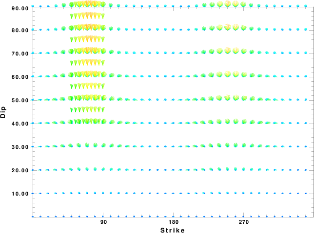
Focal mechanism sensitivity at the preferred depth. The red color indicates a very good fit to the waveforms.
Each solution is plotted as a vector at a given value of strike and dip with the angle of the vector representing the rake angle, measured, with respect to the upward vertical (N) in the figure.
|
A check on the assumed source location is possible by looking at the time shifts between the observed and predicted traces. The time shifts for waveform matching arise for several reasons:
- The origin time and epicentral distance are incorrect
- The velocity model used for the inversion is incorrect
- The velocity model used to define the P-arrival time is not the
same as the velocity model used for the waveform inversion
(assuming that the initial trace alignment is based on the
P arrival time)
Assuming only a mislocation, the time shifts are fit to a functional form:
Time_shift = A + B cos Azimuth + C Sin Azimuth
The time shifts for this inversion lead to the next figure:
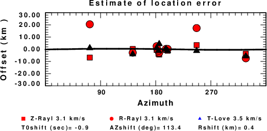
The derived shift in origin time and epicentral coordinates are given at the bottom of the figure.
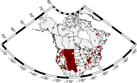
Surface-Wave Focal Mechanism
The following figure shows the stations used in the grid search for the best focal mechanism to fit the surface-wave spectral amplitudes of the Love and Rayleigh waves.
|
|
Location of broadband stations used to obtain focal mechanism from surface-wave spectral amplitudes
|
The surface-wave determined focal mechanism is shown here.
  NODAL PLANES


  STK=     165.00
  DIP=      90.00
 RAKE=    -165.00

             OR

  STK=      75.00
  DIP=      75.00
 RAKE=       0.00


DEPTH = 11.0 km

Mw = 5.09
Best Fit 0.8665 - P-T axis plot gives solutions with FIT greater than FIT90
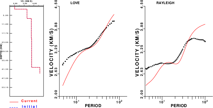
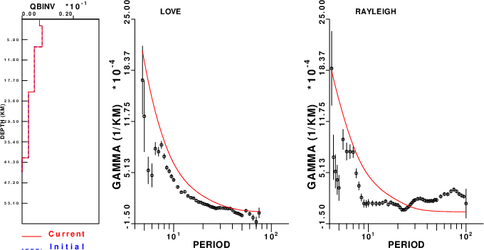
Surface-wave analysis
Surface wave analysis was performed using codes from
Computer Programs in Seismology, specifically the
multiple filter analysis program do_mft and the surface-wave
radiation pattern search program srfgrd96.
Data preparation
Digital data were collected, instrument response removed and traces converted
to Z, R an T components. Multiple filter analysis was applied to the Z and T traces to obtain the Rayleigh- and Love-wave spectral amplitudes, respectively.
These were input to the search program which examined all depths between 1 and 25 km
and all possible mechanisms.
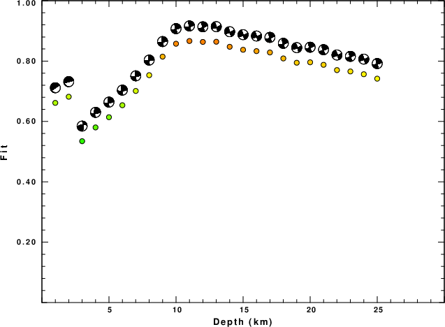
|
|
Best mechanism fit as a function of depth. The preferred depth is given above. Lower hemisphere projection
|
|
|
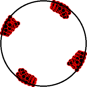
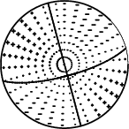
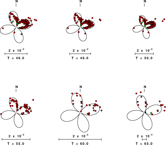
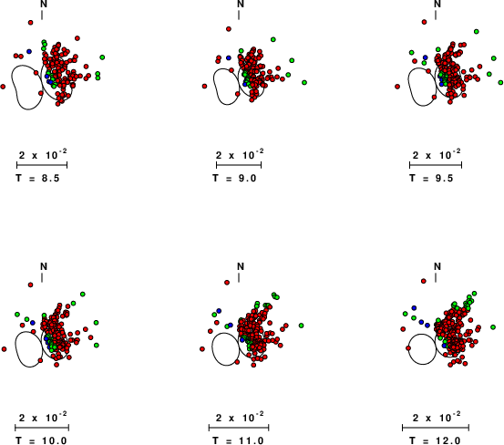
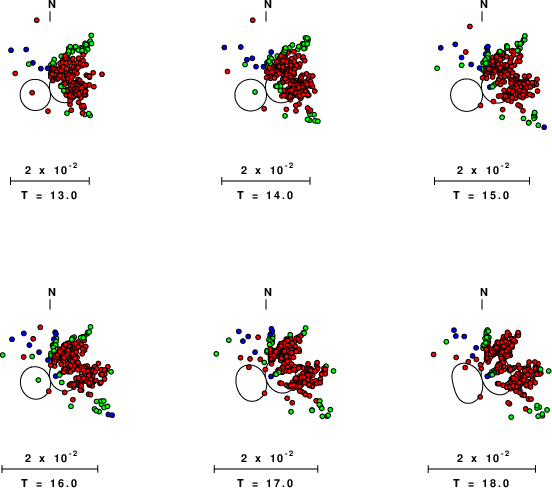
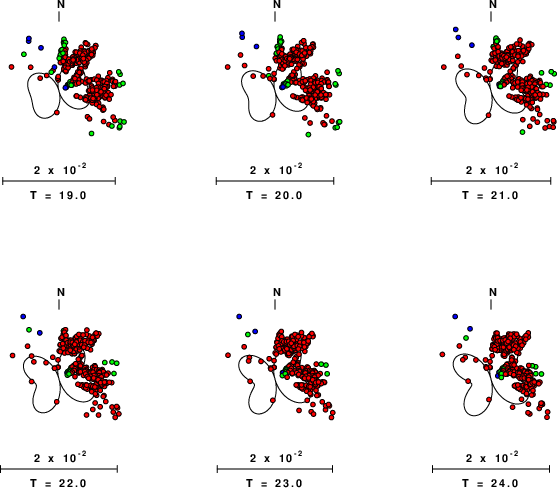
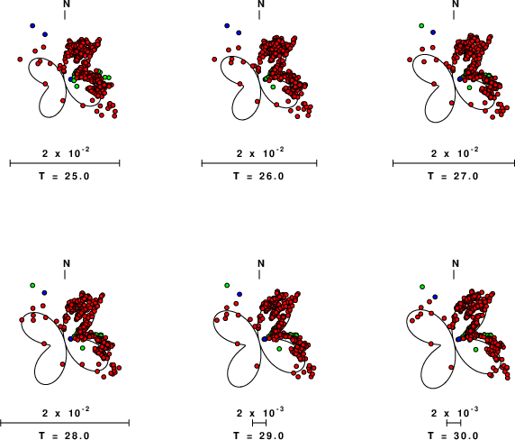
Pressure-tension axis trends. Since the surface-wave spectra search does not distinguish between P and T axes and since there is a 180 ambiguity in strike, all possible P and T axes are plotted. First motion data and waveforms will be used to select the preferred mechanism. The purpose of this plot is to provide an idea of the
possible range of solutions. The P and T-axes for all mechanisms with goodness of fit greater than 0.9 FITMAX (above) are plotted here.
|
|
|
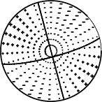
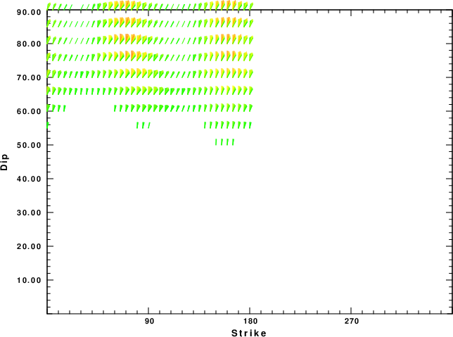
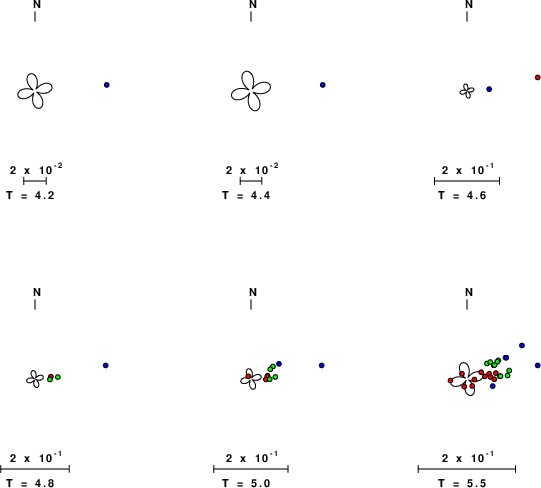
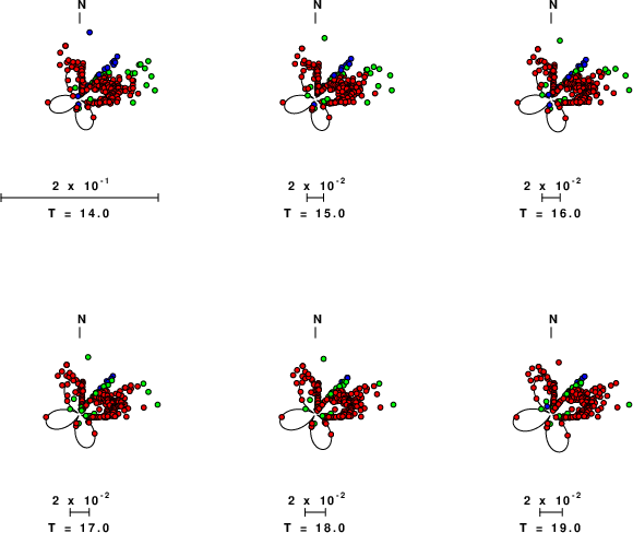
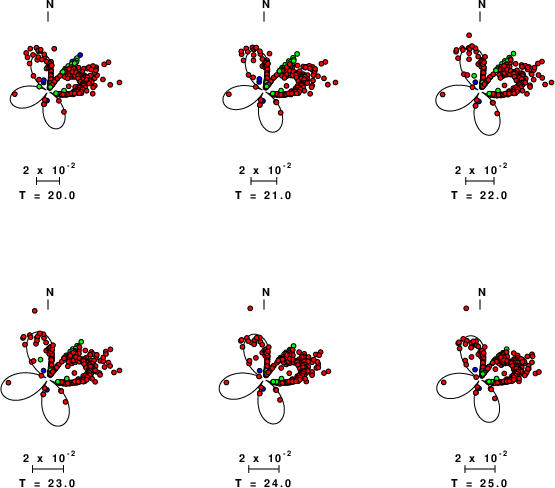
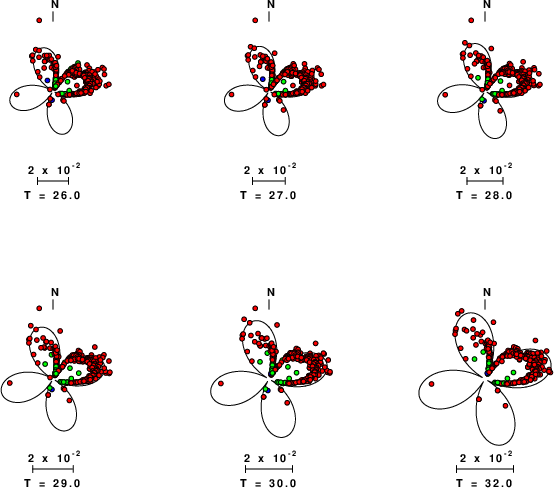
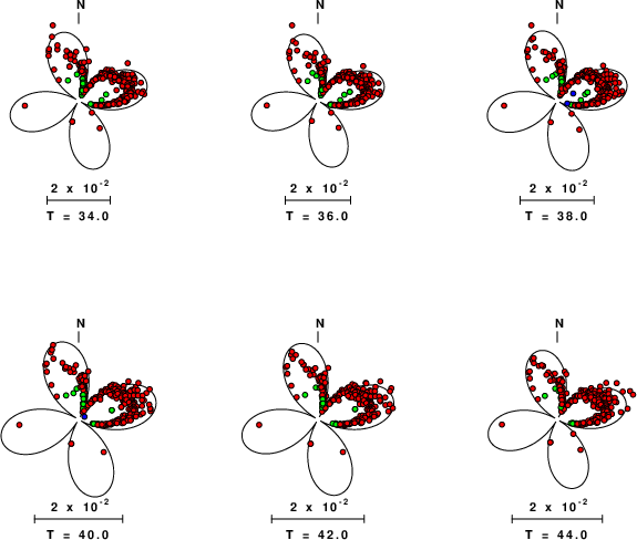
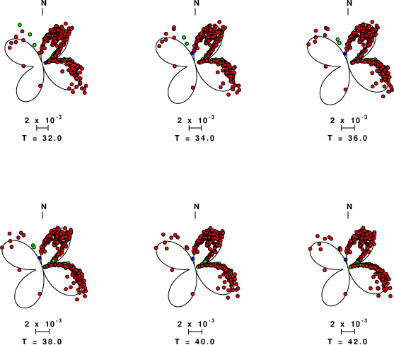
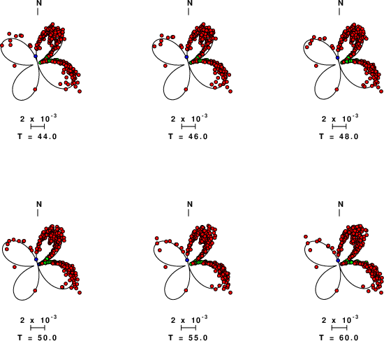
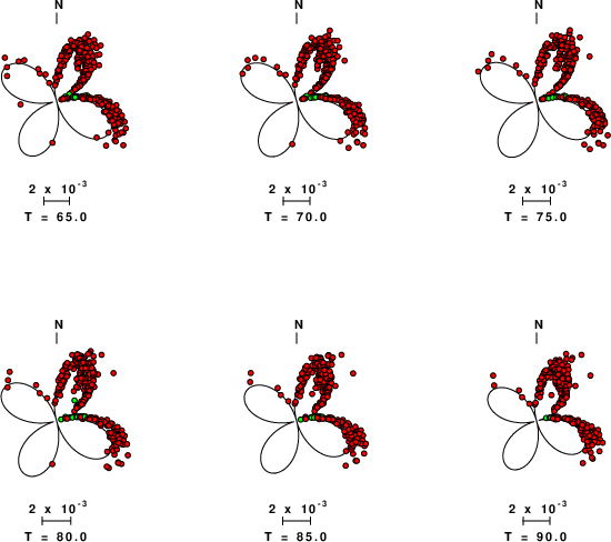
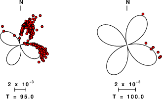
Focal mechanism sensitivity at the preferred depth. The red color indicates a very good fit to the Love and Rayleigh wave radiation patterns.
Each solution is plotted as a vector at a given value of strike and dip with the angle of the vector representing the rake angle, measured, with respect to the upward vertical (N) in the figure. Because of the symmetry of the spectral amplitude rediation patterns, only strikes from 0-180 degrees are sampled.
|
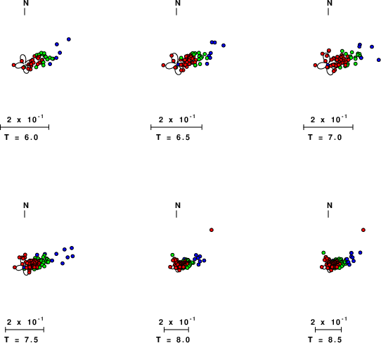
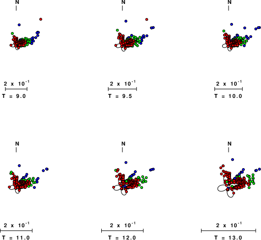
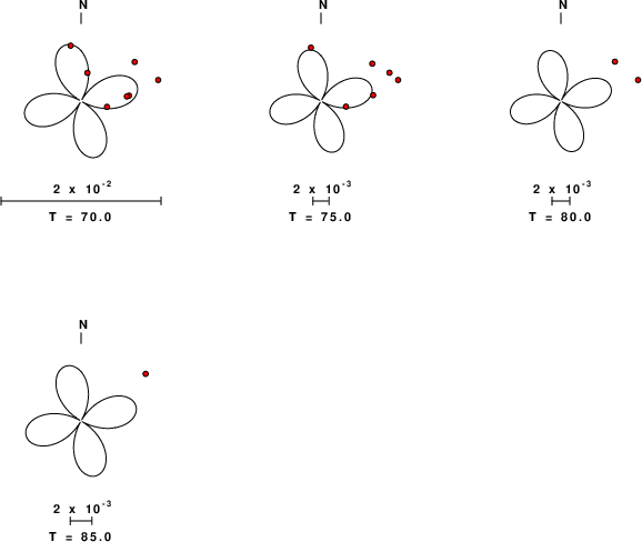
Love-wave radiation patterns
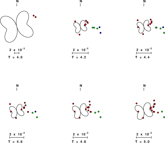
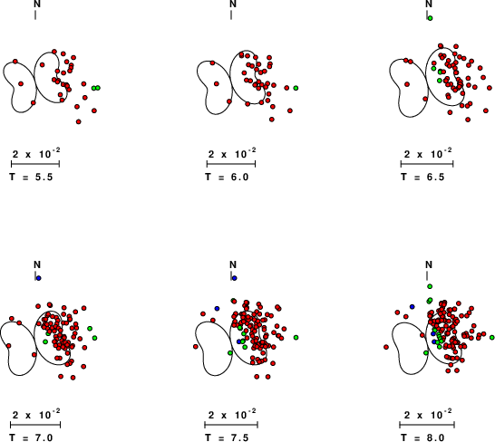
Rayleigh-wave radiation patterns