Location
Location ANSS
The ANSS event ID is usp000gmv1 and the event page is at
https://earthquake.usgs.gov/earthquakes/eventpage/usp000gmv1/executive.
2008/11/03 13:14:13 42.825 -105.182 5.0 3.5 Wyoming
Focal Mechanism
 USGS/SLU Moment Tensor Solution
 ENS  2008/11/03 13:14:13:0  42.83 -105.18   5.0 3.5 Wyoming

 Stations used:
   IU.RSSD IW.LOHW IW.PHWY IW.SMCO TA.E20A TA.E21A TA.F21A
   TA.G20A TA.G21A TA.H19A TA.H20A TA.H21A TA.H22A TA.H23A
   TA.H24A TA.I19A TA.I20A TA.I21A TA.I22A TA.I23A TA.J17A
   TA.J19A TA.J20A TA.J21A TA.J22A TA.J23A TA.K19A TA.K22A
   TA.L20A TA.L21A TA.L22A TA.L23A TA.L24A TA.M21A TA.M22A
   TA.M23A TA.M24A TA.N24A TA.N25A TA.O20A TA.O21A TA.O24A
   TA.O25A TA.P22A TA.P25A TA.Q22A TA.Q25A US.ISCO US.LAO
   US.RLMT

 Filtering commands used:
   hp c 0.02 n 3
   lp c 0.10 n 3
   br c 0.12 0.25 n 4 p 2

 Best Fitting Double Couple
  Mo = 2.57e+21 dyne-cm
  Mw = 3.54
  Z  = 18 km
  Plane   Strike  Dip  Rake
   NP1       60    73   -121
   NP2      305    35   -30
  Principal Axes:
   Axis    Value   Plunge  Azimuth
    T   2.57e+21     22     174
    N   0.00e+00     30      70
    P  -2.57e+21     51     294

 Moment Tensor: (dyne-cm)
    Component   Value
       Mxx     2.01e+21
       Mxy     1.31e+20
       Mxz    -1.41e+21
       Myy    -8.02e+20
       Myz     1.24e+21
       Mzz    -1.21e+21


                     ##############
                 ######################
              ############################
             #-----------------############
           -----------------------###########
          ---------------------------#########
         ------------------------------######--
        ----------   --------------------##-----
        ---------- P --------------------#------
       -----------   ------------------####------
       ------------------------------#######-----
       ----------------------------##########----
       -------------------------#############----
        --------------------##################--
        -----------------#####################--
         -----------##########################-
          --#################################-
           ##################################
             ###############   ############
              ############## T ###########
                 ###########   ########
                     ##############


 Global CMT Convention Moment Tensor:
      R          T          P
 -1.21e+21  -1.41e+21  -1.24e+21
 -1.41e+21   2.01e+21  -1.31e+20
 -1.24e+21  -1.31e+20  -8.02e+20


Details of the solution is found at

http://www.eas.slu.edu/eqc/eqc_mt/MECH.NA/20081103131413/index.html
|
Preferred Solution
The preferred solution from an analysis of the surface-wave spectral amplitude radiation pattern, waveform inversion or first motion observations is
      STK = 305
      DIP = 35
     RAKE = -30
       MW = 3.54
       HS = 18.0
The NDK file is 20081103131413.ndk
The waveform inversion is preferred.
Magnitudes
Given the availability of digital waveforms for determination of the moment tensor, this section documents the added processing leading to mLg, if appropriate to the region, and ML by application of the respective IASPEI formulae. As a research study, the linear distance term of the IASPEI formula
for ML is adjusted to remove a linear distance trend in residuals to give a regionally defined ML. The defined ML uses horizontal component recordings, but the same procedure is applied to the vertical components since there may be some interest in vertical component ground motions. Residual plots versus distance may indicate interesting features of ground motion scaling in some distance ranges. A residual plot of the regionalized magnitude is given as a function of distance and azimuth, since data sets may transcend different wave propagation provinces.
ML Magnitude
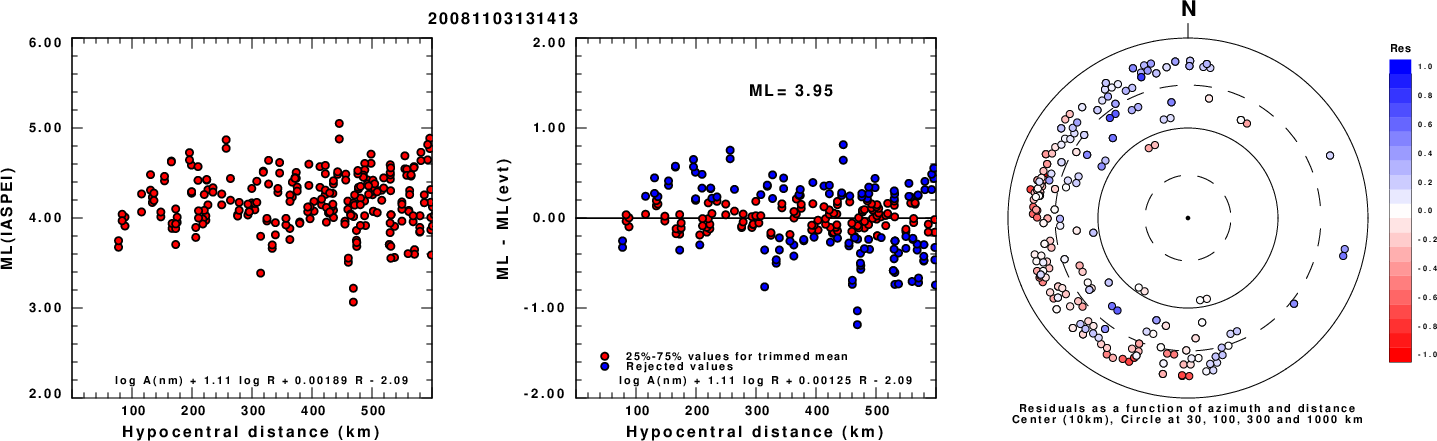
Left: ML computed using the IASPEI formula for Horizontal components. Center: ML residuals computed using a modified IASPEI formula that accounts for path specific attenuation; the values used for the trimmed mean are indicated. The ML relation used for each figure is given at the bottom of each plot.
Right: Residuals from new relation as a function of distance and azimuth.
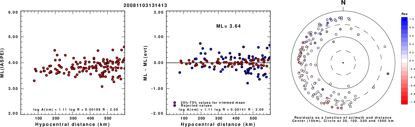
Left: ML computed using the IASPEI formula for Vertical components (research). Center: ML residuals computed using a modified IASPEI formula that accounts for path specific attenuation; the values used for the trimmed mean are indicated. The ML relation used for each figure is given at the bottom of each plot.
Right: Residuals from new relation as a function of distance and azimuth.
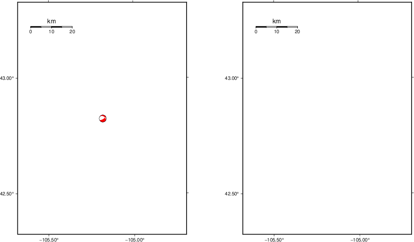
Context
The left panel of the next figure presents the focal mechanism for this earthquake (red) in the context of other nearby events (blue) in the SLU Moment Tensor Catalog. The right panel shows the inferred direction of maximum compressive stress and the type of faulting (green is strike-slip, red is normal, blue is thrust; oblique is shown by a combination of colors). Thus context plot is useful for assessing the appropriateness of the moment tensor of this event.
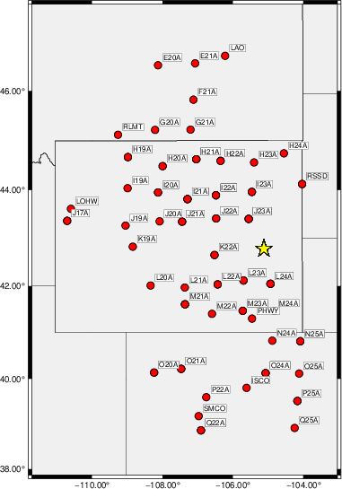
Waveform Inversion using wvfgrd96
The focal mechanism was determined using broadband seismic waveforms. The location of the event (star) and the
stations used for (red) the waveform inversion are shown in the next figure.
|
|
Location of broadband stations used for waveform inversion
|
The program wvfgrd96 was used with good traces observed at short distance to determine the focal mechanism, depth and seismic moment. This technique requires a high quality signal and well determined velocity model for the Green's functions. To the extent that these are the quality data, this type of mechanism should be preferred over the radiation pattern technique which requires the separate step of defining the pressure and tension quadrants and the correct strike.
The observed and predicted traces are filtered using the following gsac commands:
hp c 0.02 n 3
lp c 0.10 n 3
br c 0.12 0.25 n 4 p 2
The results of this grid search are as follow:
           DEPTH  STK   DIP  RAKE   MW    FIT
WVFGRD96    0.5   225    45    90   3.35 0.3452
WVFGRD96    1.0   225    45    90   3.40 0.3571
WVFGRD96    2.0   250    45    90   3.45 0.3381
WVFGRD96    3.0   335    30    25   3.48 0.3091
WVFGRD96    4.0   335    30    25   3.48 0.3438
WVFGRD96    5.0   330    30    15   3.47 0.3708
WVFGRD96    6.0   330    30    15   3.46 0.3904
WVFGRD96    7.0   325    35     5   3.46 0.4047
WVFGRD96    8.0   315    35   -20   3.46 0.4177
WVFGRD96    9.0   315    35   -20   3.46 0.4292
WVFGRD96   10.0   315    35   -20   3.49 0.4372
WVFGRD96   11.0   310    35   -25   3.50 0.4459
WVFGRD96   12.0   310    35   -30   3.50 0.4522
WVFGRD96   13.0   310    35   -30   3.51 0.4577
WVFGRD96   14.0   310    35   -25   3.51 0.4619
WVFGRD96   15.0   310    35   -25   3.52 0.4650
WVFGRD96   16.0   305    35   -30   3.53 0.4673
WVFGRD96   17.0   310    35   -25   3.53 0.4688
WVFGRD96   18.0   305    35   -30   3.54 0.4693
WVFGRD96   19.0   305    35   -30   3.55 0.4690
WVFGRD96   20.0   305    35   -30   3.58 0.4677
WVFGRD96   21.0   310    35   -25   3.59 0.4656
WVFGRD96   22.0   310    35   -25   3.60 0.4626
WVFGRD96   23.0   310    35   -25   3.60 0.4583
WVFGRD96   24.0   310    35   -25   3.61 0.4533
WVFGRD96   25.0   310    35   -25   3.62 0.4479
WVFGRD96   26.0   310    30   -25   3.63 0.4418
WVFGRD96   27.0   310    30   -20   3.64 0.4350
WVFGRD96   28.0   310    30   -20   3.64 0.4273
WVFGRD96   29.0   310    30   -20   3.65 0.4186
WVFGRD96   30.0   310    30   -20   3.66 0.4092
WVFGRD96   31.0   310    30   -20   3.67 0.3996
WVFGRD96   32.0   310    30   -20   3.67 0.3891
WVFGRD96   33.0   310    35   -20   3.68 0.3785
WVFGRD96   34.0   310    35   -20   3.69 0.3675
WVFGRD96   35.0   310    35   -25   3.69 0.3564
WVFGRD96   36.0   310    35   -20   3.69 0.3452
WVFGRD96   37.0   310    35   -20   3.70 0.3346
WVFGRD96   38.0   340    30    25   3.70 0.3262
WVFGRD96   39.0   340    30    25   3.70 0.3199
WVFGRD96   40.0   340    20    20   3.82 0.3121
WVFGRD96   41.0   340    25    25   3.83 0.3016
WVFGRD96   42.0   250    75    65   3.80 0.2933
WVFGRD96   43.0   250    75    65   3.81 0.2866
WVFGRD96   44.0   250    75    60   3.81 0.2800
WVFGRD96   45.0   250    75    60   3.81 0.2734
WVFGRD96   46.0   215    65   -65   3.86 0.2689
WVFGRD96   47.0   215    65   -65   3.87 0.2669
WVFGRD96   48.0   215    65   -60   3.87 0.2647
WVFGRD96   49.0   215    65   -60   3.88 0.2631
WVFGRD96   50.0   215    65   -60   3.88 0.2612
The best solution is
WVFGRD96 18.0 305 35 -30 3.54 0.4693
The mechanism corresponding to the best fit is
|
|
Figure 1. Waveform inversion focal mechanism
|
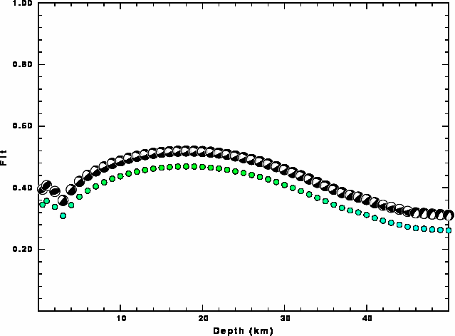
The best fit as a function of depth is given in the following figure:
|
|
Figure 2. Depth sensitivity for waveform mechanism
|
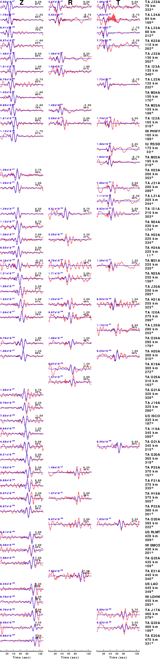
The comparison of the observed and predicted waveforms is given in the next figure. The red traces are the observed and the blue are the predicted.
Each observed-predicted component is plotted to the same scale and peak amplitudes are indicated by the numbers to the left of each trace. A pair of numbers is given in black at the right of each predicted traces. The upper number it the time shift required for maximum correlation between the observed and predicted traces. This time shift is required because the synthetics are not computed at exactly the same distance as the observed, the velocity model used in the predictions may not be perfect and the epicentral parameters may be be off.
A positive time shift indicates that the prediction is too fast and should be delayed to match the observed trace (shift to the right in this figure). A negative value indicates that the prediction is too slow. The lower number gives the percentage of variance reduction to characterize the individual goodness of fit (100% indicates a perfect fit).
The bandpass filter used in the processing and for the display was
hp c 0.02 n 3
lp c 0.10 n 3
br c 0.12 0.25 n 4 p 2
|
|
Figure 3. Waveform comparison for selected depth. Red: observed; Blue - predicted. The time shift with respect to the model prediction is indicated. The percent of fit is also indicated. The time scale is relative to the first trace sample.
|
|
|
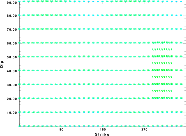
Focal mechanism sensitivity at the preferred depth. The red color indicates a very good fit to the waveforms.
Each solution is plotted as a vector at a given value of strike and dip with the angle of the vector representing the rake angle, measured, with respect to the upward vertical (N) in the figure.
|
A check on the assumed source location is possible by looking at the time shifts between the observed and predicted traces. The time shifts for waveform matching arise for several reasons:
- The origin time and epicentral distance are incorrect
- The velocity model used for the inversion is incorrect
- The velocity model used to define the P-arrival time is not the
same as the velocity model used for the waveform inversion
(assuming that the initial trace alignment is based on the
P arrival time)
Assuming only a mislocation, the time shifts are fit to a functional form:
Time_shift = A + B cos Azimuth + C Sin Azimuth
The time shifts for this inversion lead to the next figure:
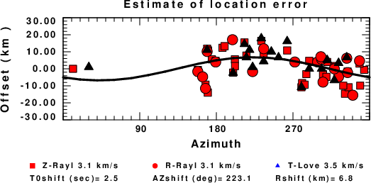
The derived shift in origin time and epicentral coordinates are given at the bottom of the figure.
Velocity Model
The CUS.model used for the waveform synthetic seismograms and for the surface wave eigenfunctions and dispersion is as follows
(The format is in the model96 format of Computer Programs in Seismology).
MODEL.01
CUS Model with Q from simple gamma values
ISOTROPIC
KGS
FLAT EARTH
1-D
CONSTANT VELOCITY
LINE08
LINE09
LINE10
LINE11
  H(KM) VP(KM/S) VS(KM/S) RHO(GM/CC)   QP   QS  ETAP  ETAS  FREFP  FREFS
  1.0000  5.0000  2.8900  2.5000 0.172E-02 0.387E-02 0.00  0.00  1.00  1.00
  9.0000  6.1000  3.5200  2.7300 0.160E-02 0.363E-02 0.00  0.00  1.00  1.00
 10.0000  6.4000  3.7000  2.8200 0.149E-02 0.336E-02 0.00  0.00  1.00  1.00
 20.0000  6.7000  3.8700  2.9020 0.000E-04 0.000E-04 0.00  0.00  1.00  1.00
  0.0000  8.1500  4.7000  3.3640 0.194E-02 0.431E-02 0.00  0.00  1.00  1.00
Last Changed Sun Apr 28 01:02:35 PM CDT 2024