The ANSS event ID is usp000ghd9 and the event page is at https://earthquake.usgs.gov/earthquakes/eventpage/usp000ghd9/executive.
2008/09/20 05:16:11 63.588 -129.029 10.0 5.2 NWT, Canada
 USGS/SLU Moment Tensor Solution
 ENS  2008/09/20 05:16:11:0  63.59 -129.03  10.0 5.2 NWT, Canada

 Stations used:
   AK.PNL AT.SKAG CN.CTLN CN.DAWY CN.DLBC CN.FNBB CN.GALN
   CN.ILKN CN.INK US.EGAK

 Filtering commands used:
   hp c 0.02 n 3
   lp c 0.10 n 3

 Best Fitting Double Couple
  Mo = 6.68e+23 dyne-cm
  Mw = 5.15
  Z  = 12 km
  Plane   Strike  Dip  Rake
   NP1      250    75    20
   NP2      155    71   164
  Principal Axes:
   Axis    Value   Plunge  Azimuth
    T   6.68e+23     25     113
    N   0.00e+00     65     285
    P  -6.68e+23      3      22

 Moment Tensor: (dyne-cm)
    Component   Value
       Mxx    -4.91e+23
       Mxy    -4.28e+23
       Mxz    -1.30e+23
       Myy     3.77e+23
       Myz     2.20e+23
       Mzz     1.14e+23


                     ------------ P
                 ##--------------   ---
              #####-----------------------
             ######------------------------
           ########--------------------------
          #########---------------------------
         ###########---------------------------
        ############-----------------###########
        #############---------##################
       ###############---########################
       #############--###########################
       ##########------##########################
       #######----------#########################
        ###--------------################   ####
        #-----------------############### T ####
         ------------------##############   ###
          ------------------##################
           -------------------###############
             ------------------############
              -------------------#########
                 ------------------####
                     --------------


 Global CMT Convention Moment Tensor:
      R          T          P
  1.14e+23  -1.30e+23  -2.20e+23
 -1.30e+23  -4.91e+23   4.28e+23
 -2.20e+23   4.28e+23   3.77e+23


Details of the solution is found at

http://www.eas.slu.edu/eqc/eqc_mt/MECH.NA/20080920051611/index.html
|
      STK = 250
      DIP = 75
     RAKE = 20
       MW = 5.15
       HS = 12.0
The NDK file is 20080920051611.ndk The waveform inversion is preferred.
|
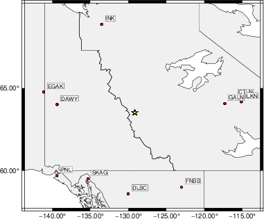
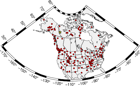
The focal mechanism was determined using broadband seismic waveforms. The location of the event (star) and the stations used for (red) the waveform inversion are shown in the next figure.
|
|
|
The program wvfgrd96 was used with good traces observed at short distance to determine the focal mechanism, depth and seismic moment. This technique requires a high quality signal and well determined velocity model for the Green's functions. To the extent that these are the quality data, this type of mechanism should be preferred over the radiation pattern technique which requires the separate step of defining the pressure and tension quadrants and the correct strike.
The observed and predicted traces are filtered using the following gsac commands:
hp c 0.02 n 3
lp c 0.10 n 3
The results of this grid search are as follow:
           DEPTH  STK   DIP  RAKE   MW    FIT
WVFGRD96    0.5    65    80   -25   4.95 0.4615
WVFGRD96    1.0    65    80   -25   4.98 0.4757
WVFGRD96    2.0    60    70   -10   5.03 0.4859
WVFGRD96    3.0    60    80    20   5.07 0.4905
WVFGRD96    4.0   245    75    30   5.08 0.5024
WVFGRD96    5.0   245    75    25   5.09 0.5180
WVFGRD96    6.0   245    75    25   5.10 0.5303
WVFGRD96    7.0   250    70    25   5.09 0.5358
WVFGRD96    8.0   245    75    20   5.12 0.5514
WVFGRD96    9.0   250    75    20   5.11 0.5570
WVFGRD96   10.0   245    75    20   5.15 0.5709
WVFGRD96   11.0   250    75    20   5.14 0.5706
WVFGRD96   12.0   250    75    20   5.15 0.5724
WVFGRD96   13.0   250    75    15   5.16 0.5714
WVFGRD96   14.0   250    75    15   5.17 0.5656
WVFGRD96   15.0   250    75    15   5.18 0.5631
WVFGRD96   16.0   250    75    15   5.19 0.5538
WVFGRD96   17.0   250    75    15   5.20 0.5429
WVFGRD96   18.0   245    80    15   5.23 0.5349
WVFGRD96   19.0   245    80    15   5.24 0.5200
WVFGRD96   20.0   240    85    15   5.28 0.5053
WVFGRD96   21.0   245    80    15   5.26 0.4905
WVFGRD96   22.0    65    75     0   5.25 0.4760
WVFGRD96   23.0    60    75    -5   5.28 0.4612
WVFGRD96   24.0    60    75   -10   5.28 0.4468
WVFGRD96   25.0    60    75   -10   5.28 0.4320
WVFGRD96   26.0    60    75   -10   5.28 0.4208
WVFGRD96   27.0    60    75   -10   5.29 0.4096
WVFGRD96   28.0    60    75   -10   5.29 0.3988
WVFGRD96   29.0    60    75   -10   5.30 0.3886
WVFGRD96   30.0    60    75   -10   5.30 0.3787
WVFGRD96   31.0   330    80    10   5.32 0.3680
WVFGRD96   32.0   330    80    10   5.33 0.3614
WVFGRD96   33.0   330    80    10   5.34 0.3540
WVFGRD96   34.0   330    80    10   5.35 0.3462
WVFGRD96   35.0   330    80    10   5.36 0.3378
WVFGRD96   36.0   330    80    10   5.37 0.3295
WVFGRD96   37.0    60    75   -10   5.37 0.3229
WVFGRD96   38.0    60    80   -10   5.39 0.3168
WVFGRD96   39.0    60    80    -5   5.42 0.3107
WVFGRD96   40.0    60    75   -10   5.45 0.3041
WVFGRD96   41.0    60    75    -5   5.47 0.2998
WVFGRD96   42.0    60    80   -10   5.48 0.2948
WVFGRD96   43.0    60    80     5   5.50 0.2890
WVFGRD96   44.0    60    80     5   5.51 0.2828
WVFGRD96   45.0    60    80     5   5.52 0.2761
WVFGRD96   46.0    65    80    10   5.50 0.2690
WVFGRD96   47.0    65    80    10   5.51 0.2634
WVFGRD96   48.0    60    85     5   5.55 0.2576
WVFGRD96   49.0   240    90   -10   5.55 0.2504
WVFGRD96   50.0    60    85     5   5.56 0.2454
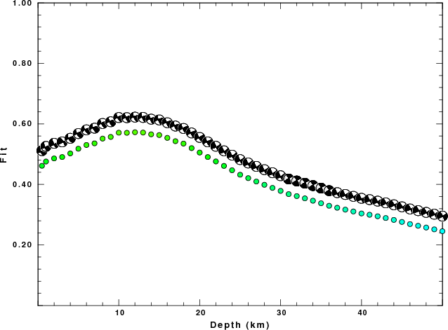
The best solution is
WVFGRD96 12.0 250 75 20 5.15 0.5724
The mechanism corresponding to the best fit is
|
|
|
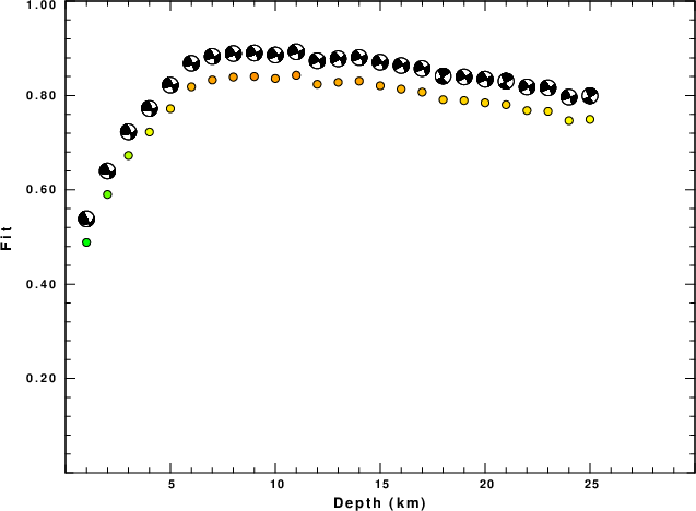
The best fit as a function of depth is given in the following figure:
|
|
|
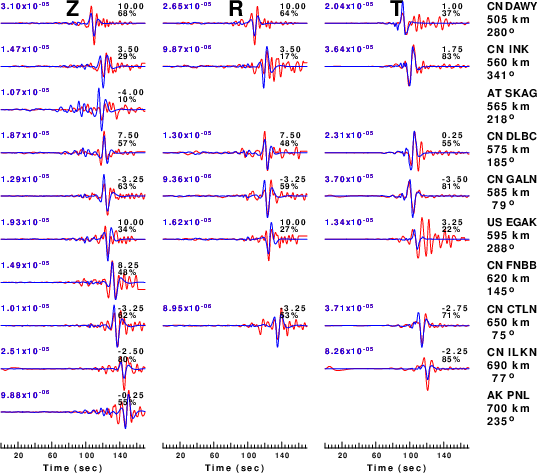
The comparison of the observed and predicted waveforms is given in the next figure. The red traces are the observed and the blue are the predicted. Each observed-predicted component is plotted to the same scale and peak amplitudes are indicated by the numbers to the left of each trace. A pair of numbers is given in black at the right of each predicted traces. The upper number it the time shift required for maximum correlation between the observed and predicted traces. This time shift is required because the synthetics are not computed at exactly the same distance as the observed, the velocity model used in the predictions may not be perfect and the epicentral parameters may be be off. A positive time shift indicates that the prediction is too fast and should be delayed to match the observed trace (shift to the right in this figure). A negative value indicates that the prediction is too slow. The lower number gives the percentage of variance reduction to characterize the individual goodness of fit (100% indicates a perfect fit).
The bandpass filter used in the processing and for the display was
hp c 0.02 n 3
lp c 0.10 n 3
|
| Figure 3. Waveform comparison for selected depth. Red: observed; Blue - predicted. The time shift with respect to the model prediction is indicated. The percent of fit is also indicated. The time scale is relative to the first trace sample. |
|
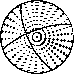
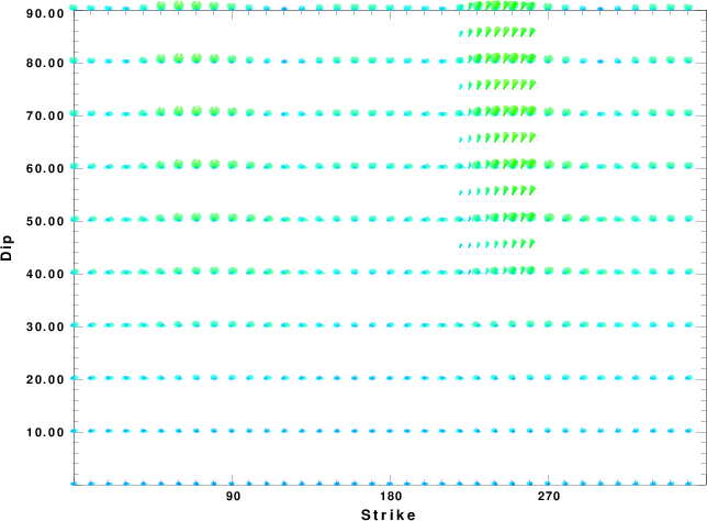
| Focal mechanism sensitivity at the preferred depth. The red color indicates a very good fit to the waveforms. Each solution is plotted as a vector at a given value of strike and dip with the angle of the vector representing the rake angle, measured, with respect to the upward vertical (N) in the figure. |
A check on the assumed source location is possible by looking at the time shifts between the observed and predicted traces. The time shifts for waveform matching arise for several reasons:
Time_shift = A + B cos Azimuth + C Sin Azimuth
The time shifts for this inversion lead to the next figure:
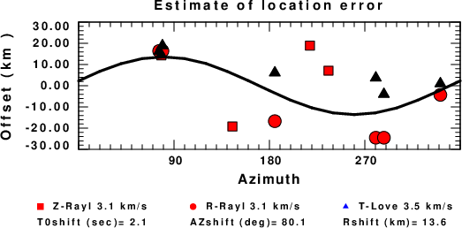
The derived shift in origin time and epicentral coordinates are given at the bottom of the figure.
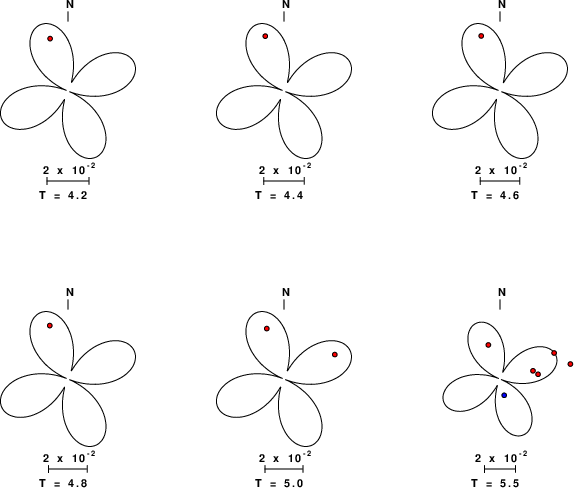
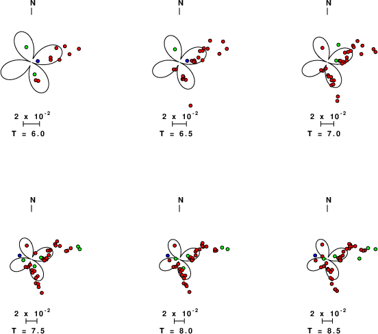
The following figure shows the stations used in the grid search for the best focal mechanism to fit the surface-wave spectral amplitudes of the Love and Rayleigh waves.
|
|
|
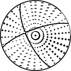
The surface-wave determined focal mechanism is shown here.
  NODAL PLANES


  STK=     249.99
  DIP=      75.00
 RAKE=      19.99

             OR

  STK=     154.61
  DIP=      70.72
 RAKE=     164.08


DEPTH = 11.0 km

Mw = 5.21
Best Fit 0.8420 - P-T axis plot gives solutions with FIT greater than FIT90
 |
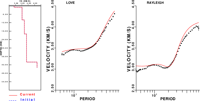
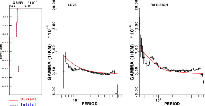
Surface wave analysis was performed using codes from Computer Programs in Seismology, specifically the multiple filter analysis program do_mft and the surface-wave radiation pattern search program srfgrd96.
Digital data were collected, instrument response removed and traces converted
to Z, R an T components. Multiple filter analysis was applied to the Z and T traces to obtain the Rayleigh- and Love-wave spectral amplitudes, respectively.
These were input to the search program which examined all depths between 1 and 25 km
and all possible mechanisms.
|
|
|
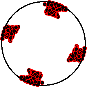
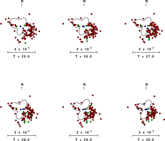
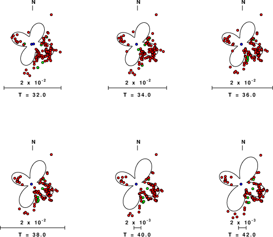
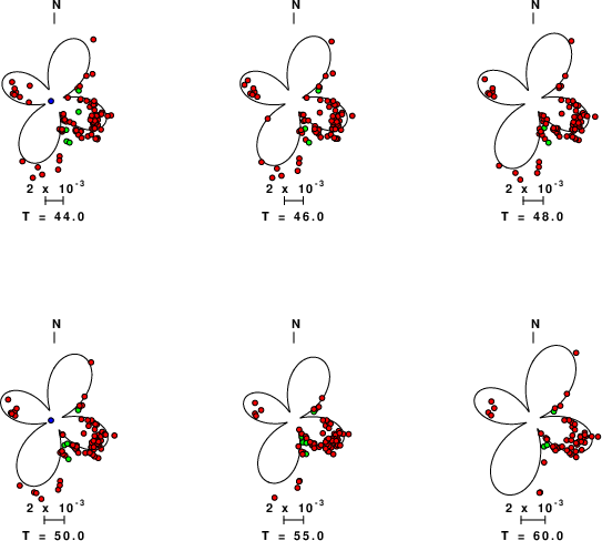
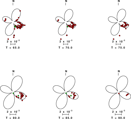
|
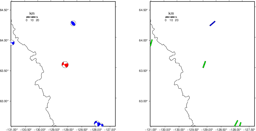
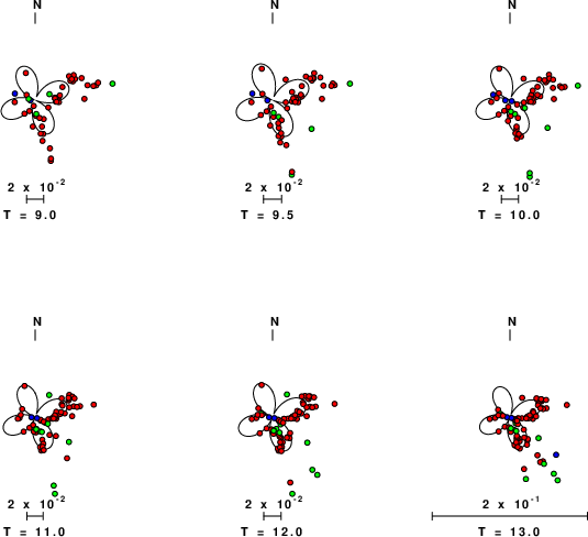
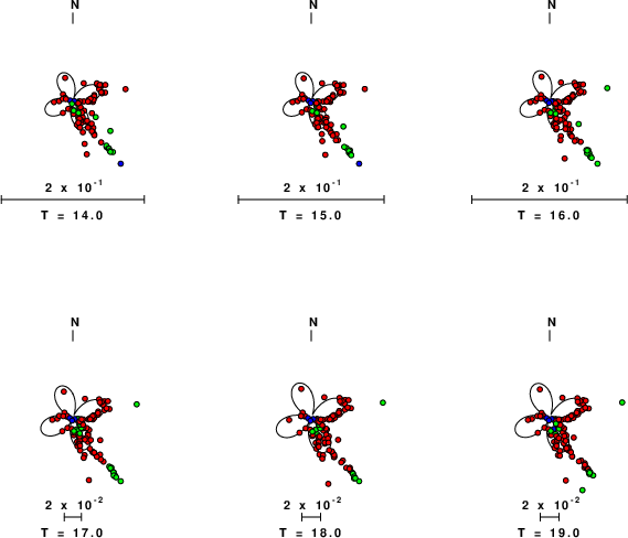
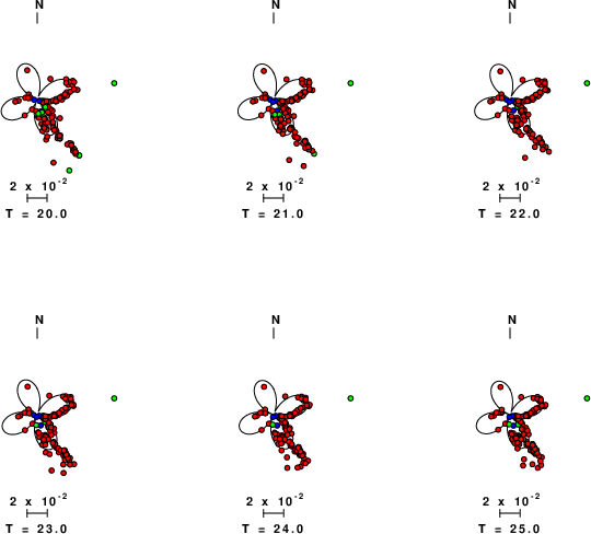
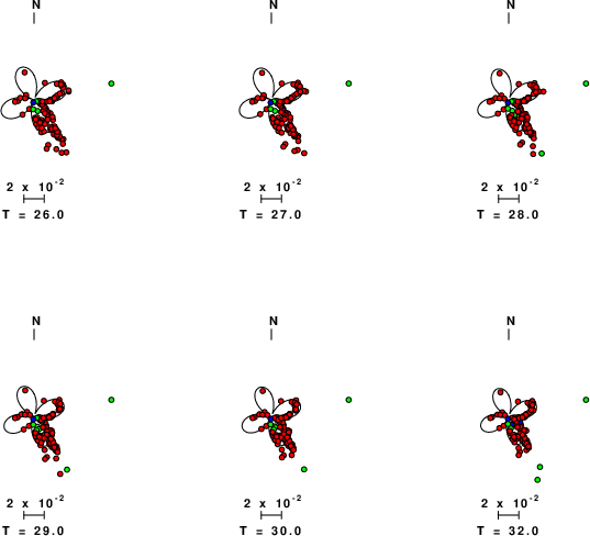
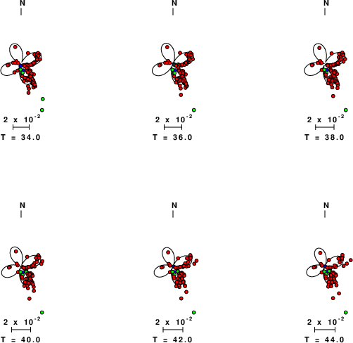
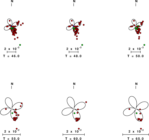
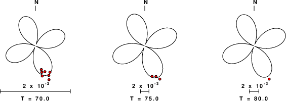
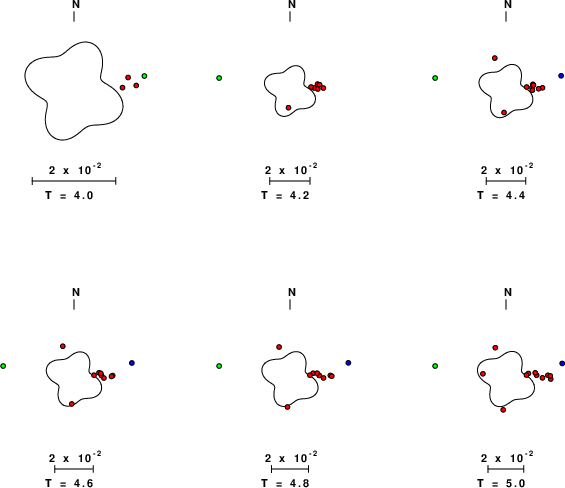
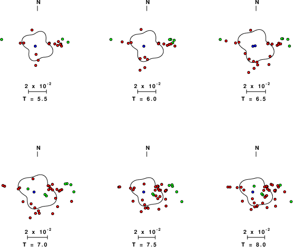
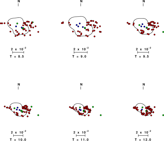
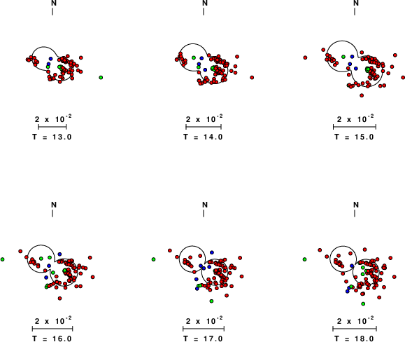
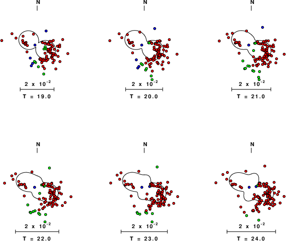
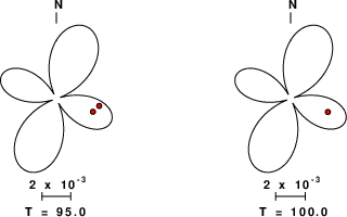
| Pressure-tension axis trends. Since the surface-wave spectra search does not distinguish between P and T axes and since there is a 180 ambiguity in strike, all possible P and T axes are plotted. First motion data and waveforms will be used to select the preferred mechanism. The purpose of this plot is to provide an idea of the possible range of solutions. The P and T-axes for all mechanisms with goodness of fit greater than 0.9 FITMAX (above) are plotted here. |
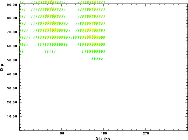
|
| Focal mechanism sensitivity at the preferred depth. The red color indicates a very good fit to the Love and Rayleigh wave radiation patterns. Each solution is plotted as a vector at a given value of strike and dip with the angle of the vector representing the rake angle, measured, with respect to the upward vertical (N) in the figure. Because of the symmetry of the spectral amplitude rediation patterns, only strikes from 0-180 degrees are sampled. |
|
|
The CUS.model used for the waveform synthetic seismograms and for the surface wave eigenfunctions and dispersion is as follows (The format is in the model96 format of Computer Programs in Seismology).
MODEL.01
CUS Model with Q from simple gamma values
ISOTROPIC
KGS
FLAT EARTH
1-D
CONSTANT VELOCITY
LINE08
LINE09
LINE10
LINE11
  H(KM) VP(KM/S) VS(KM/S) RHO(GM/CC)   QP   QS  ETAP  ETAS  FREFP  FREFS
  1.0000  5.0000  2.8900  2.5000 0.172E-02 0.387E-02 0.00  0.00  1.00  1.00
  9.0000  6.1000  3.5200  2.7300 0.160E-02 0.363E-02 0.00  0.00  1.00  1.00
 10.0000  6.4000  3.7000  2.8200 0.149E-02 0.336E-02 0.00  0.00  1.00  1.00
 20.0000  6.7000  3.8700  2.9020 0.000E-04 0.000E-04 0.00  0.00  1.00  1.00
  0.0000  8.1500  4.7000  3.3640 0.194E-02 0.431E-02 0.00  0.00  1.00  1.00