Location
Location ANSS
The ANSS event ID is ci14383980 and the event page is at
https://earthquake.usgs.gov/earthquakes/eventpage/ci14383980/executive.
2008/07/29 18:42:15 33.949 -117.766 15.5 5.44 California
Focal Mechanism
 USGS/SLU Moment Tensor Solution
 ENS  2008/07/29 18:42:15:0  33.95 -117.77  15.5 5.4 California

 Stations used:
   CI.BAR CI.GLA CI.GSC CI.ISA CI.MWC CI.OSI II.PFO NN.WCN
   TA.109C TA.113A TA.114A TA.116A TA.117A TA.214A TA.216A
   TA.217A

 Filtering commands used:
   hp c 0.02 n 3
   lp c 0.10 n 3

 Best Fitting Double Couple
  Mo = 1.29e+24 dyne-cm
  Mw = 5.34
  Z  = 17 km
  Plane   Strike  Dip  Rake
   NP1      289    58   138
   NP2       45    55    40
  Principal Axes:
   Axis    Value   Plunge  Azimuth
    T   1.29e+24     51     255
    N   0.00e+00     39      79
    P  -1.29e+24      2     348

 Moment Tensor: (dyne-cm)
    Component   Value
       Mxx    -1.20e+24
       Mxy     3.89e+23
       Mxz    -2.00e+23
       Myy     4.19e+23
       Myz    -6.01e+23
       Mzz     7.78e+23


                     - P ----------
                 -----   --------------
              ----------------------------
             ------------------------------
           --------------------------------##
          ---------------------------------###
         --#################---------------####
        #########################---------######
        #############################----#######
       #################################-########
       #################################--#######
       ##########   ###################-----#####
       ########## T #################--------####
        #########   ################-----------#
        ##########################-------------#
         #######################---------------
          ####################----------------
           ################------------------
             #########---------------------
              ----------------------------
                 ----------------------
                     --------------


 Global CMT Convention Moment Tensor:
      R          T          P
  7.78e+23  -2.00e+23   6.01e+23
 -2.00e+23  -1.20e+24  -3.89e+23
  6.01e+23  -3.89e+23   4.19e+23


Details of the solution is found at

http://www.eas.slu.edu/eqc/eqc_mt/MECH.NA/20080729184215/index.html
|
Preferred Solution
The preferred solution from an analysis of the surface-wave spectral amplitude radiation pattern, waveform inversion or first motion observations is
      STK = 45
      DIP = 55
     RAKE = 40
       MW = 5.34
       HS = 17.0
The NDK file is 20080729184215.ndk
The waveform inversion is preferred.
Moment Tensor Comparison
The following compares this source inversion to those provided by others. The purpose is to look for major differences and also to note slight differences that might be inherent to the processing procedure. For completeness the USGS/SLU solution is repeated from above.
| SLU |
USGSMT |
SCAL |
 USGS/SLU Moment Tensor Solution
 ENS  2008/07/29 18:42:15:0  33.95 -117.77  15.5 5.4 California

 Stations used:
   CI.BAR CI.GLA CI.GSC CI.ISA CI.MWC CI.OSI II.PFO NN.WCN
   TA.109C TA.113A TA.114A TA.116A TA.117A TA.214A TA.216A
   TA.217A

 Filtering commands used:
   hp c 0.02 n 3
   lp c 0.10 n 3

 Best Fitting Double Couple
  Mo = 1.29e+24 dyne-cm
  Mw = 5.34
  Z  = 17 km
  Plane   Strike  Dip  Rake
   NP1      289    58   138
   NP2       45    55    40
  Principal Axes:
   Axis    Value   Plunge  Azimuth
    T   1.29e+24     51     255
    N   0.00e+00     39      79
    P  -1.29e+24      2     348

 Moment Tensor: (dyne-cm)
    Component   Value
       Mxx    -1.20e+24
       Mxy     3.89e+23
       Mxz    -2.00e+23
       Myy     4.19e+23
       Myz    -6.01e+23
       Mzz     7.78e+23


                     - P ----------
                 -----   --------------
              ----------------------------
             ------------------------------
           --------------------------------##
          ---------------------------------###
         --#################---------------####
        #########################---------######
        #############################----#######
       #################################-########
       #################################--#######
       ##########   ###################-----#####
       ########## T #################--------####
        #########   ################-----------#
        ##########################-------------#
         #######################---------------
          ####################----------------
           ################------------------
             #########---------------------
              ----------------------------
                 ----------------------
                     --------------


 Global CMT Convention Moment Tensor:
      R          T          P
  7.78e+23  -2.00e+23   6.01e+23
 -2.00e+23  -1.20e+24  -3.89e+23
  6.01e+23  -3.89e+23   4.19e+23


Details of the solution is found at

http://www.eas.slu.edu/eqc/eqc_mt/MECH.NA/20080729184215/index.html
|
USGS Centroid Moment Tensor Solution

 08/07/29 18:42:15.07
 GREATER LOS ANGELES AREA, CALIF.
 Epicenter:  33.733 -117.940
 MW 5.4

 USGS CENTROID MOMENT TENSOR
 08/07/29 18:42:46.50
 Centroid:   34.645 -117.325
 Depth  22         No. of sta:110
 Moment Tensor;   Scale 10**17 Nm
   Mrr= 1.02       Mtt=-1.45
   Mpp= 0.43       Mrt=-0.76
   Mrp=-0.03       Mtp=-0.77
  Principal axes:
   T  Val=  1.28  Plg=65  Azm=219
   N        0.62      20       76
   P       -1.90      13      341

 Best Double Couple:Mo=1.6*10**17
  NP1:Strike= 46 Dip=36 Slip=  54
  NP2:       268     62       113

               -------
          --   ------------
        ---- P --------------
      ------   ----------------
    ---------------------------##
   -----------------------------##
   -----------------------------##
  -------####################--####
  ---##########################---#
  ############################-----
  ############   #############-----
  ############ T ############------
   ###########   ##########-------
   #######################--------
    ###################----------
      ##############-----------
        ---------------------
          -----------------
               -------
|
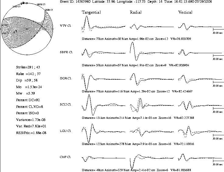
SCSN Moment Tensor Solution Message **

REAL-TIME SOLUTION: OPERATOR REVIEWED
Reviewed On: 07/29/2008 19:7:4

Inversion Method: Complete Waveform
Number of Stations used: 6
Stations: CI.VTV CI.SBPX CI.DGR CI.SCI2 CI.LGU CI.CHF

Real-Time Solution:
-------------------
Event ID    : 14383980
Magnitude   : 5.76
Depth (km)  : 12.4
Origin Time :  07/29/2008 18:42:15:690
Latitude    : 33.96
Longitude   : -117.75
Further Information at: http://pasadena.wr.usgs.gov/recenteqs/Quakes/ci14383980.htm

SCSN Moment Tensor Solution:
----------------------------
Moment Magnitude     : 5.39
Depth (km)           : 14
Variance Reduction(%): 78.18
Quality Factor       : A
   (A : Mw, MT good enough for distribution)
   (B : Mw only good enough for distribution)
   (C : Solution needs review before distribution)


Best Fitting Double Couple and CLVD Solution:
---------------------------------------------------

Moment Tensor: Scale = 10**21 Dyne-cm
    Component   Value
       Mxx      -1450
       Mxy      495
       Mxz      -198
       Myy      602
       Myz      -689
       Mzz      844

Best Fitting Double Couple Solution:
--------------------------------------------------
 Moment Tensor: Scale = 10**24 Dyne-cm
    Component   Value
       Mxx     -1.417
       Mxy      0.490
       Mxz     -0.190
       Myy      0.585
       Myz     -0.739
       Mzz      0.832

 Principle Axes:
    Axis    Value   Plunge   Azimuth
      T     1.531      48      257
      N     0.000      42       78
      P    -1.531       1      347

 Best Fitting Double-Couple:
    Mo = 1.53E+24 Dyne-cm
    Plane   Strike   Rake   Dip
     NP1      291     142    59
     NP2       43      37    58

 Moment Magnitude = 5.39


                  P -------
              ---   -------------
           -------------------------
         -----------------------------
       ------------------------------###
      -------------------------------####
     --------------------------------#####
    ####################------------#######
    #########################-------#######
   #############################---#########
   ###############################-#########
   ##########   #################----#######
   ########## T ###############--------#####
   ##########   ##############----------####
    ########################--------------#
    ######################-----------------
     ###################------------------
      ###############--------------------
       ###########----------------------
         ###--------------------------
           -------------------------
              -------------------
                    -------

     Lower Hemisphere Equiangle Projection

=============  Station Information ==============

Name       Distance     Azimuth     VR      ZCore
-------------------------------------------------
CI.VTV       77.054     30.048   76.836     12.00
CI.SBPX      56.326     57.420   82.856      9.00
CI.DGR       76.703    116.423   82.425     12.00
CI.SCI2     131.529    214.497   62.227     16.00
CI.LGU      122.621    278.069   72.110     16.00
CI.CHF       48.604    328.515   81.956      6.00
|
|
|
Magnitudes
Given the availability of digital waveforms for determination of the moment tensor, this section documents the added processing leading to mLg, if appropriate to the region, and ML by application of the respective IASPEI formulae. As a research study, the linear distance term of the IASPEI formula
for ML is adjusted to remove a linear distance trend in residuals to give a regionally defined ML. The defined ML uses horizontal component recordings, but the same procedure is applied to the vertical components since there may be some interest in vertical component ground motions. Residual plots versus distance may indicate interesting features of ground motion scaling in some distance ranges. A residual plot of the regionalized magnitude is given as a function of distance and azimuth, since data sets may transcend different wave propagation provinces.
ML Magnitude
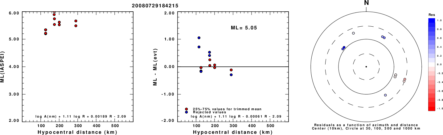
Left: ML computed using the IASPEI formula for Horizontal components. Center: ML residuals computed using a modified IASPEI formula that accounts for path specific attenuation; the values used for the trimmed mean are indicated. The ML relation used for each figure is given at the bottom of each plot.
Right: Residuals from new relation as a function of distance and azimuth.
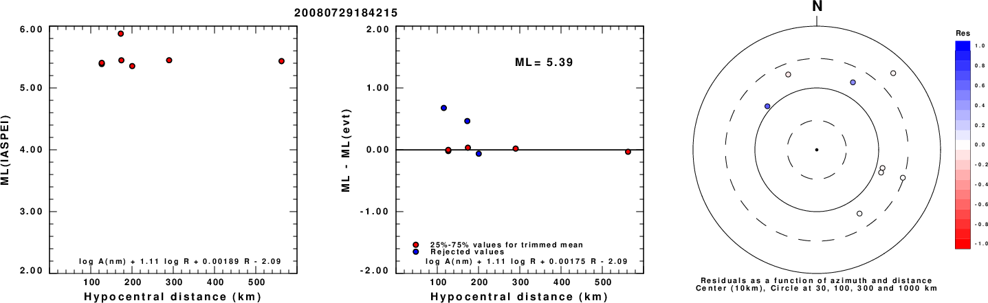
Left: ML computed using the IASPEI formula for Vertical components (research). Center: ML residuals computed using a modified IASPEI formula that accounts for path specific attenuation; the values used for the trimmed mean are indicated. The ML relation used for each figure is given at the bottom of each plot.
Right: Residuals from new relation as a function of distance and azimuth.
Context
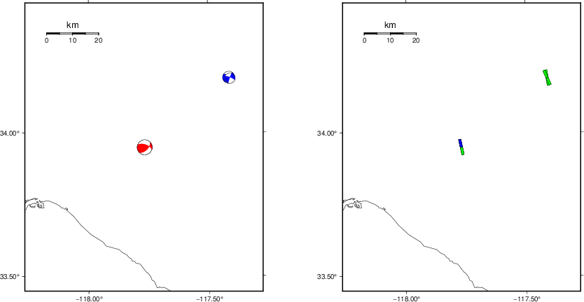
The left panel of the next figure presents the focal mechanism for this earthquake (red) in the context of other nearby events (blue) in the SLU Moment Tensor Catalog. The right panel shows the inferred direction of maximum compressive stress and the type of faulting (green is strike-slip, red is normal, blue is thrust; oblique is shown by a combination of colors). Thus context plot is useful for assessing the appropriateness of the moment tensor of this event.
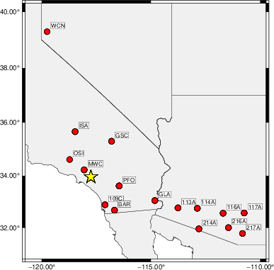
Waveform Inversion using wvfgrd96
The focal mechanism was determined using broadband seismic waveforms. The location of the event (star) and the
stations used for (red) the waveform inversion are shown in the next figure.
|
|
Location of broadband stations used for waveform inversion
|
The program wvfgrd96 was used with good traces observed at short distance to determine the focal mechanism, depth and seismic moment. This technique requires a high quality signal and well determined velocity model for the Green's functions. To the extent that these are the quality data, this type of mechanism should be preferred over the radiation pattern technique which requires the separate step of defining the pressure and tension quadrants and the correct strike.
The observed and predicted traces are filtered using the following gsac commands:
hp c 0.02 n 3
lp c 0.10 n 3
The results of this grid search are as follow:
           DEPTH  STK   DIP  RAKE   MW    FIT
WVFGRD96    0.5    80    40   -90   4.79 0.2780
WVFGRD96    1.0    80    45   -80   4.80 0.2450
WVFGRD96    2.0    80    40   -90   4.97 0.3307
WVFGRD96    3.0   100    35   -60   4.99 0.2756
WVFGRD96    4.0   215    75   -50   4.96 0.3062
WVFGRD96    5.0   215    80   -45   4.98 0.3454
WVFGRD96    6.0   215    80   -45   5.01 0.3834
WVFGRD96    7.0   215    80   -40   5.03 0.4174
WVFGRD96    8.0    40    80    45   5.10 0.4499
WVFGRD96    9.0    40    75    45   5.13 0.4882
WVFGRD96   10.0    45    65    45   5.17 0.5266
WVFGRD96   11.0    50    50    50   5.23 0.5711
WVFGRD96   12.0    50    50    50   5.26 0.6110
WVFGRD96   13.0    50    50    50   5.28 0.6414
WVFGRD96   14.0    50    50    45   5.30 0.6637
WVFGRD96   15.0    45    55    40   5.31 0.6796
WVFGRD96   16.0    45    55    40   5.33 0.6889
WVFGRD96   17.0    45    55    40   5.34 0.6946
WVFGRD96   18.0    45    55    40   5.35 0.6940
WVFGRD96   19.0    45    55    40   5.37 0.6874
WVFGRD96   20.0    40    60    35   5.37 0.6784
WVFGRD96   21.0    45    60    40   5.38 0.6662
WVFGRD96   22.0    45    60    40   5.39 0.6532
WVFGRD96   23.0    45    60    40   5.40 0.6363
WVFGRD96   24.0    40    65    40   5.39 0.6191
WVFGRD96   25.0    40    65    40   5.40 0.5987
WVFGRD96   26.0    40    65    40   5.40 0.5773
WVFGRD96   27.0    45    65    45   5.40 0.5539
WVFGRD96   28.0    40    70    45   5.40 0.5304
WVFGRD96   29.0    40    70    45   5.40 0.5056
The best solution is
WVFGRD96 17.0 45 55 40 5.34 0.6946
The mechanism corresponding to the best fit is
|
|
Figure 1. Waveform inversion focal mechanism
|
The best fit as a function of depth is given in the following figure:
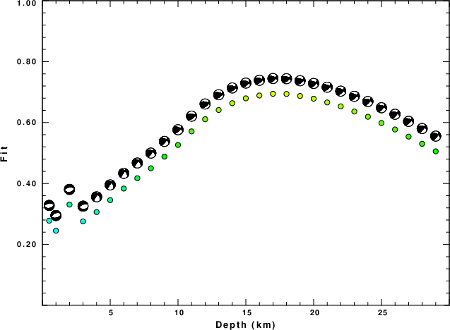
|
|
Figure 2. Depth sensitivity for waveform mechanism
|
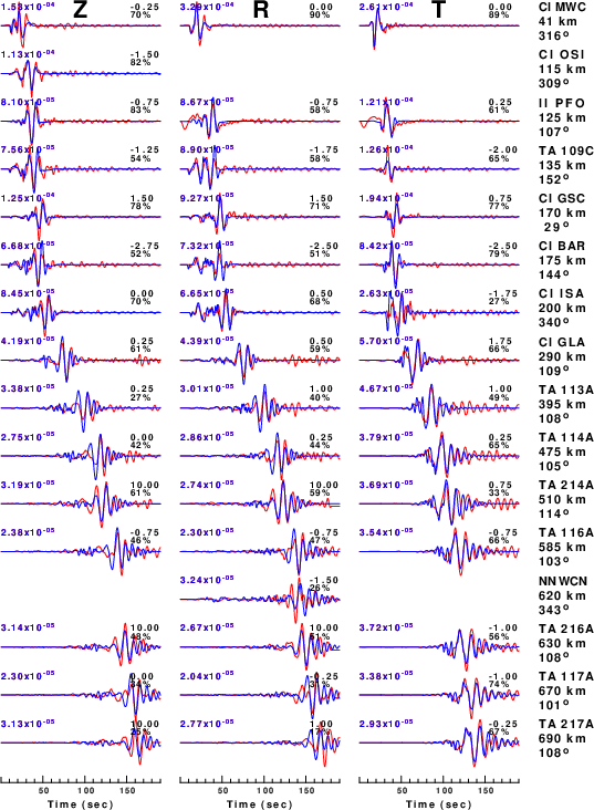
The comparison of the observed and predicted waveforms is given in the next figure. The red traces are the observed and the blue are the predicted.
Each observed-predicted component is plotted to the same scale and peak amplitudes are indicated by the numbers to the left of each trace. A pair of numbers is given in black at the right of each predicted traces. The upper number it the time shift required for maximum correlation between the observed and predicted traces. This time shift is required because the synthetics are not computed at exactly the same distance as the observed, the velocity model used in the predictions may not be perfect and the epicentral parameters may be be off.
A positive time shift indicates that the prediction is too fast and should be delayed to match the observed trace (shift to the right in this figure). A negative value indicates that the prediction is too slow. The lower number gives the percentage of variance reduction to characterize the individual goodness of fit (100% indicates a perfect fit).
The bandpass filter used in the processing and for the display was
hp c 0.02 n 3
lp c 0.10 n 3
|
|
Figure 3. Waveform comparison for selected depth. Red: observed; Blue - predicted. The time shift with respect to the model prediction is indicated. The percent of fit is also indicated. The time scale is relative to the first trace sample.
|
|
|
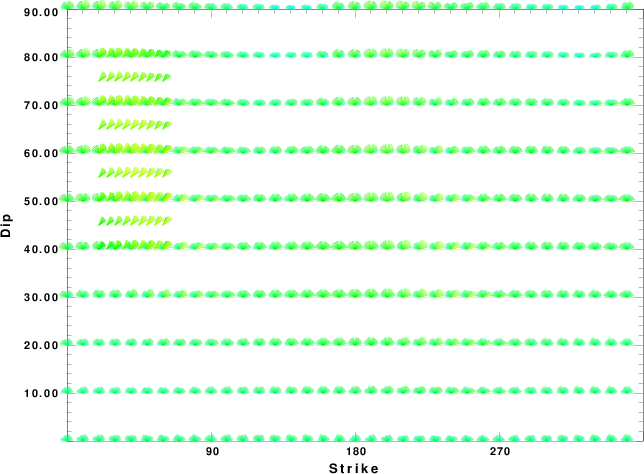
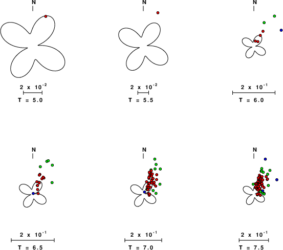
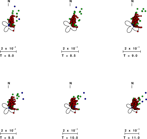
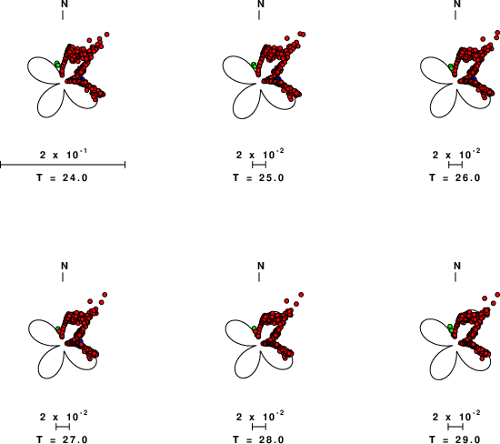
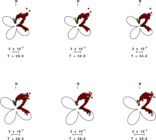
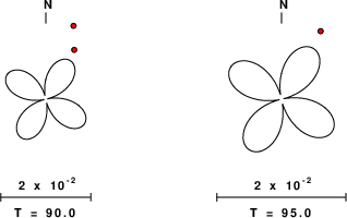
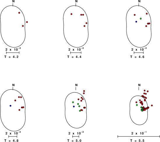
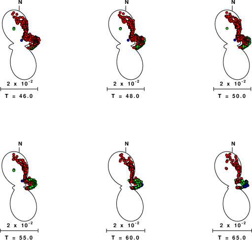
Focal mechanism sensitivity at the preferred depth. The red color indicates a very good fit to the waveforms.
Each solution is plotted as a vector at a given value of strike and dip with the angle of the vector representing the rake angle, measured, with respect to the upward vertical (N) in the figure.
|
A check on the assumed source location is possible by looking at the time shifts between the observed and predicted traces. The time shifts for waveform matching arise for several reasons:
- The origin time and epicentral distance are incorrect
- The velocity model used for the inversion is incorrect
- The velocity model used to define the P-arrival time is not the
same as the velocity model used for the waveform inversion
(assuming that the initial trace alignment is based on the
P arrival time)
Assuming only a mislocation, the time shifts are fit to a functional form:
Time_shift = A + B cos Azimuth + C Sin Azimuth
The time shifts for this inversion lead to the next figure:
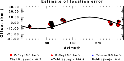
The derived shift in origin time and epicentral coordinates are given at the bottom of the figure.
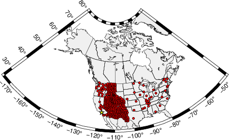
Surface-Wave Focal Mechanism
The following figure shows the stations used in the grid search for the best focal mechanism to fit the surface-wave spectral amplitudes of the Love and Rayleigh waves.
|
|
Location of broadband stations used to obtain focal mechanism from surface-wave spectral amplitudes
|
The surface-wave determined focal mechanism is shown here.
  NODAL PLANES


  STK=     279.72
  DIP=      54.61
 RAKE=     119.84

             OR

  STK=      54.99
  DIP=      45.00
 RAKE=      55.00


DEPTH = 13.0 km

Mw = 5.46
Best Fit 0.8748 - P-T axis plot gives solutions with FIT greater than FIT90
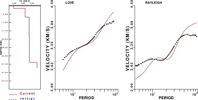
Surface-wave analysis
Surface wave analysis was performed using codes from
Computer Programs in Seismology, specifically the
multiple filter analysis program do_mft and the surface-wave
radiation pattern search program srfgrd96.
Data preparation
Digital data were collected, instrument response removed and traces converted
to Z, R an T components. Multiple filter analysis was applied to the Z and T traces to obtain the Rayleigh- and Love-wave spectral amplitudes, respectively.
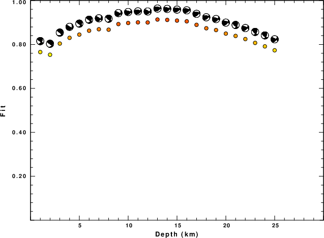
These were input to the search program which examined all depths between 1 and 25 km
and all possible mechanisms.
|
|
Best mechanism fit as a function of depth. The preferred depth is given above. Lower hemisphere projection
|

|
|
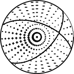
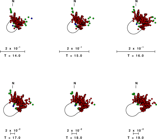
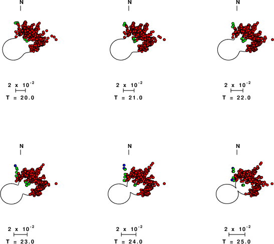
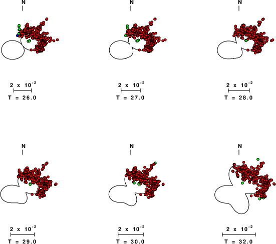
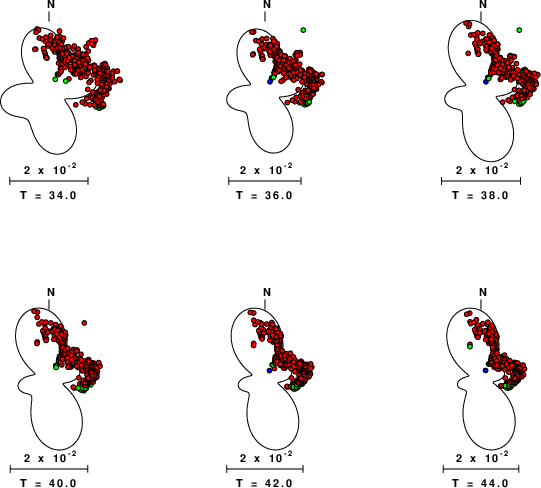
Pressure-tension axis trends. Since the surface-wave spectra search does not distinguish between P and T axes and since there is a 180 ambiguity in strike, all possible P and T axes are plotted. First motion data and waveforms will be used to select the preferred mechanism. The purpose of this plot is to provide an idea of the
possible range of solutions. The P and T-axes for all mechanisms with goodness of fit greater than 0.9 FITMAX (above) are plotted here.
|
|
|
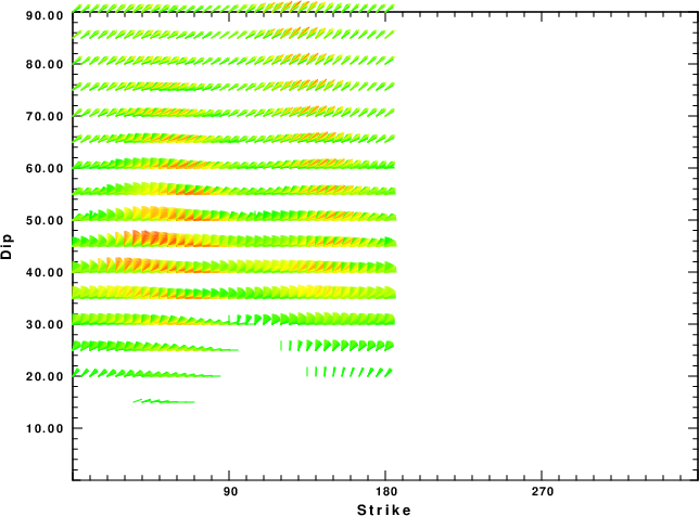
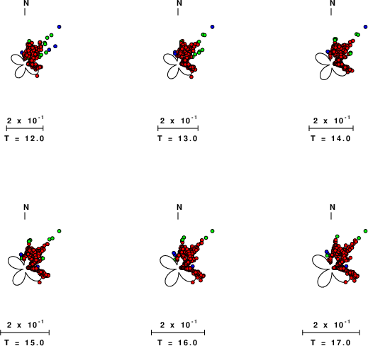
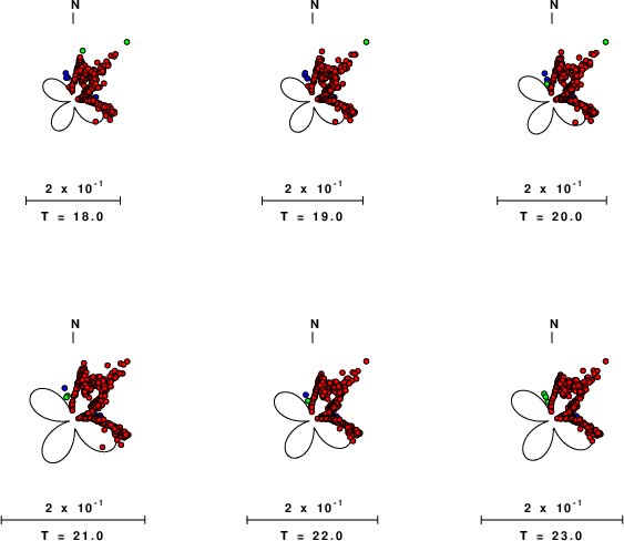
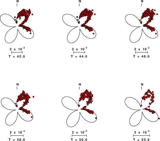
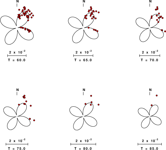
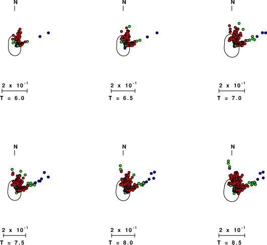
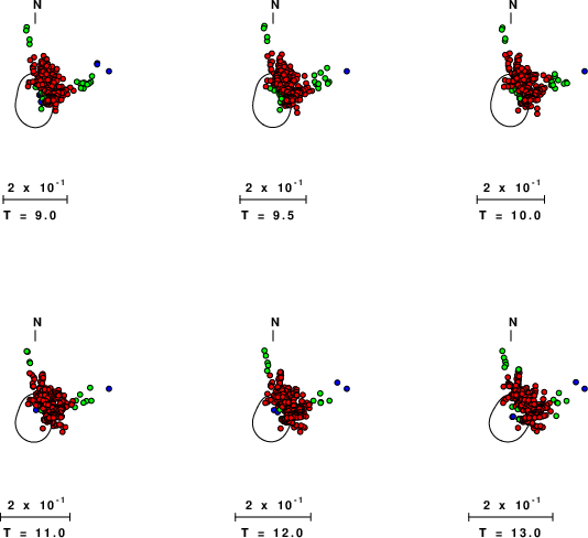
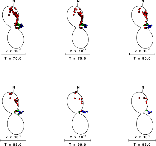
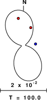
Focal mechanism sensitivity at the preferred depth. The red color indicates a very good fit to the Love and Rayleigh wave radiation patterns.
Each solution is plotted as a vector at a given value of strike and dip with the angle of the vector representing the rake angle, measured, with respect to the upward vertical (N) in the figure. Because of the symmetry of the spectral amplitude rediation patterns, only strikes from 0-180 degrees are sampled.
|
Love-wave radiation patterns
Rayleigh-wave radiation patterns