Location
Location ANSS
The ANSS event ID is ci10320621 and the event page is at
https://earthquake.usgs.gov/earthquakes/eventpage/ci10320621/executive.
2008/04/26 06:40:10 38.610 -119.133 3.5 4.7 Nevada
Focal Mechanism
 USGS/SLU Moment Tensor Solution
 ENS  2008/04/26 06:40:10:0  38.61 -119.13   3.5 4.7 Nevada

 Stations used:
   BK.CMB BK.HUMO BK.MCCM BK.SAO BK.WDC CI.ADO CI.BBR CI.BFS
   CI.CHF CI.CIA CI.CWC CI.DAN CI.EDW2 CI.FUR CI.GRA CI.GSC
   CI.ISA CI.LRL CI.MLAC CI.MPM CI.MWC CI.PASC CI.RCT CI.RPV
   CI.RRX CI.SDD CI.SHO CI.SLA CI.SVD CI.TIN CI.TUQ CI.VCS
   CI.VES CI.VTV NN.WCN TA.G04A TA.G06A TA.G07A TA.G08A
   TA.G09A TA.G10A TA.H04A TA.H06A TA.H08A TA.H09A TA.H11A
   TA.H12A TA.I07A TA.I09A TA.I10A TA.I11A TA.I12A TA.I13A
   TA.J08A TA.J09A TA.J10A TA.J11A TA.J12A TA.J13A TA.J14A
   TA.K05A TA.K10A TA.K11A TA.K12A TA.K13A TA.K14A TA.L10A
   TA.L11A TA.L12A TA.L13A TA.L14A TA.L15A TA.M10A TA.M11A
   TA.M12A TA.M13A TA.M14A TA.M15A TA.N10A TA.N11A TA.N12A
   TA.N13A TA.N14A TA.O10A TA.O11A TA.O12A TA.O13A TA.O15A
   TA.P10A TA.P11A TA.P12A TA.P13A TA.P14A TA.P15A TA.Q10A
   TA.Q11A TA.Q12A TA.Q13A TA.Q14A TA.Q15A TA.R10A TA.R11A
   TA.R12A TA.R13A TA.R14A TA.R15A TA.S10A TA.S11A TA.S12A
   TA.S13A TA.S14A TA.S15A TA.T11A TA.T12A TA.T13A TA.T14A
   TA.U10A TA.U11A TA.U12A TA.U13A TA.U14A TA.V11A TA.V12A
   TA.V13A TA.W12A US.BMO US.DUG US.ELK US.HLID US.WVOR

 Filtering commands used:
   cut o DIST/3.3 -40 o DIST/3.3 +50
   rtr
   taper w 0.1
   hp c 0.03 n 3
   lp c 0.07 n 3

 Best Fitting Double Couple
  Mo = 2.92e+23 dyne-cm
  Mw = 4.91
  Z  = 8 km
  Plane   Strike  Dip  Rake
   NP1      240    80    15
   NP2      147    75   170
  Principal Axes:
   Axis    Value   Plunge  Azimuth
    T   2.92e+23     18     104
    N   0.00e+00     72     273
    P  -2.92e+23      3      13

 Moment Tensor: (dyne-cm)
    Component   Value
       Mxx    -2.60e+23
       Mxy    -1.28e+23
       Mxz    -3.70e+22
       Myy     2.34e+23
       Myz     7.79e+22
       Mzz     2.58e+22


                     ---------- P -
                 --------------   -----
              ###-------------------------
             ####--------------------------
           #######---------------------------
          #########--------------------------#
         ##########--------------------########
        ############---------------#############
        #############----------#################
       ###############------#####################
       ################--########################
       ###############--#########################
       ############------##################   ###
        ########-----------################ T ##
        ######--------------###############   ##
         ###-----------------##################
          ---------------------###############
           ----------------------############
             ---------------------#########
              -----------------------#####
                 ----------------------
                     --------------


 Global CMT Convention Moment Tensor:
      R          T          P
  2.58e+22  -3.70e+22  -7.79e+22
 -3.70e+22  -2.60e+23   1.28e+23
 -7.79e+22   1.28e+23   2.34e+23


Details of the solution is found at

http://www.eas.slu.edu/eqc/eqc_mt/MECH.NA/20080426064010/index.html
|
Preferred Solution
The preferred solution from an analysis of the surface-wave spectral amplitude radiation pattern, waveform inversion or first motion observations is
      STK = 240
      DIP = 80
     RAKE = 15
       MW = 4.91
       HS = 8.0
The NDK file is 20080426064010.ndk
The waveform inversion is preferred.
Moment Tensor Comparison
The following compares this source inversion to those provided by others. The purpose is to look for major differences and also to note slight differences that might be inherent to the processing procedure. For completeness the USGS/SLU solution is repeated from above.
| SLU |
GCMT |
UCB |
 USGS/SLU Moment Tensor Solution
 ENS  2008/04/26 06:40:10:0  38.61 -119.13   3.5 4.7 Nevada

 Stations used:
   BK.CMB BK.HUMO BK.MCCM BK.SAO BK.WDC CI.ADO CI.BBR CI.BFS
   CI.CHF CI.CIA CI.CWC CI.DAN CI.EDW2 CI.FUR CI.GRA CI.GSC
   CI.ISA CI.LRL CI.MLAC CI.MPM CI.MWC CI.PASC CI.RCT CI.RPV
   CI.RRX CI.SDD CI.SHO CI.SLA CI.SVD CI.TIN CI.TUQ CI.VCS
   CI.VES CI.VTV NN.WCN TA.G04A TA.G06A TA.G07A TA.G08A
   TA.G09A TA.G10A TA.H04A TA.H06A TA.H08A TA.H09A TA.H11A
   TA.H12A TA.I07A TA.I09A TA.I10A TA.I11A TA.I12A TA.I13A
   TA.J08A TA.J09A TA.J10A TA.J11A TA.J12A TA.J13A TA.J14A
   TA.K05A TA.K10A TA.K11A TA.K12A TA.K13A TA.K14A TA.L10A
   TA.L11A TA.L12A TA.L13A TA.L14A TA.L15A TA.M10A TA.M11A
   TA.M12A TA.M13A TA.M14A TA.M15A TA.N10A TA.N11A TA.N12A
   TA.N13A TA.N14A TA.O10A TA.O11A TA.O12A TA.O13A TA.O15A
   TA.P10A TA.P11A TA.P12A TA.P13A TA.P14A TA.P15A TA.Q10A
   TA.Q11A TA.Q12A TA.Q13A TA.Q14A TA.Q15A TA.R10A TA.R11A
   TA.R12A TA.R13A TA.R14A TA.R15A TA.S10A TA.S11A TA.S12A
   TA.S13A TA.S14A TA.S15A TA.T11A TA.T12A TA.T13A TA.T14A
   TA.U10A TA.U11A TA.U12A TA.U13A TA.U14A TA.V11A TA.V12A
   TA.V13A TA.W12A US.BMO US.DUG US.ELK US.HLID US.WVOR

 Filtering commands used:
   cut o DIST/3.3 -40 o DIST/3.3 +50
   rtr
   taper w 0.1
   hp c 0.03 n 3
   lp c 0.07 n 3

 Best Fitting Double Couple
  Mo = 2.92e+23 dyne-cm
  Mw = 4.91
  Z  = 8 km
  Plane   Strike  Dip  Rake
   NP1      240    80    15
   NP2      147    75   170
  Principal Axes:
   Axis    Value   Plunge  Azimuth
    T   2.92e+23     18     104
    N   0.00e+00     72     273
    P  -2.92e+23      3      13

 Moment Tensor: (dyne-cm)
    Component   Value
       Mxx    -2.60e+23
       Mxy    -1.28e+23
       Mxz    -3.70e+22
       Myy     2.34e+23
       Myz     7.79e+22
       Mzz     2.58e+22


                     ---------- P -
                 --------------   -----
              ###-------------------------
             ####--------------------------
           #######---------------------------
          #########--------------------------#
         ##########--------------------########
        ############---------------#############
        #############----------#################
       ###############------#####################
       ################--########################
       ###############--#########################
       ############------##################   ###
        ########-----------################ T ##
        ######--------------###############   ##
         ###-----------------##################
          ---------------------###############
           ----------------------############
             ---------------------#########
              -----------------------#####
                 ----------------------
                     --------------


 Global CMT Convention Moment Tensor:
      R          T          P
  2.58e+22  -3.70e+22  -7.79e+22
 -3.70e+22  -2.60e+23   1.28e+23
 -7.79e+22   1.28e+23   2.34e+23


Details of the solution is found at

http://www.eas.slu.edu/eqc/eqc_mt/MECH.NA/20080426064010/index.html
|
April 26, 2008, NEVADA, MW=5.0

Meredith Nettles

CENTROID-MOMENT-TENSOR  SOLUTION
GCMT EVENT:     C200804260640A
DATA: IU CU II IC G  GE
L.P.BODY WAVES: 34S,  41C, T= 40
SURFACE WAVES:  71S, 128C, T= 50
TIMESTAMP:      Q-20080426172124
CENTROID LOCATION:
ORIGIN TIME:      06:40:15.1 0.2
LAT:39.57N 0.02;LON:119.91W 0.02
DEP: 15.4  1.1;TRIANG HDUR:  0.8
MOMENT TENSOR: SCALE 10**23 D-CM
RR=-1.010 0.136; TT=-2.980 0.105
PP= 3.980 0.126; RT= 0.206 0.368
RP= 0.029 0.316; TP= 1.680 0.103
PRINCIPAL AXES:
1.(T) VAL=  4.365;PLG= 1;AZM=283
2.(N)      -0.995;    85;     22
3.(P)      -3.380;     5;    193
BEST DBLE.COUPLE:M0= 3.87*10**23
NP1: STRIKE=328;DIP=86;SLIP=-177
NP2: STRIKE=238;DIP=87;SLIP=  -4

            -----------
        #------------------
      ####-------------------
    ########-------------------
   ##########-----------------##
  ############-------------######
   ############---------#########
 T ##############----#############
   ###############################
 ##############----###############
 ###########--------##############
  #######------------############
  #####---------------###########
   #-------------------#########
    --------------------#######
      -------------------####
        ----   -----------#
             P --------
|
This is a preliminary NCSS moment tensor solution for the event located
10 km WSW of Verdi-Mogul, NV; 39.4687N 120.0587W; Z=0.1km;  ML=4.94;
(USGS/UCB Joint Notification System) on  04/26/2008 06:40:14:070 UTC.
Other information about this event can be viewed at:
http://earthquake.usgs.gov/recenteqsus/Quakes/nc40216182.php

Reviewed by:
Achung
UCB Seismological Laboratory

Inversion method:   complete waveform
Stations used:      CI.TIN BK.ORV BK.WDC BK.YBH BK.BKS BK.HELL

 Berkeley Moment Tensor Solution

 Best Fitting Double-Couple:
    Mo = 3.40E+23 Dyne-cm
    Mw = 4.96
    Z  = 5 km
    Plane   Strike   Rake   Dip
     NP1       60      25    85
     NP2      328     174    65

 Event Date/Time:  04/26/2008 06:40:14:070
 Event ID:        40216182


                            -----------
                      -----------------------
                  -------------------------------
               #####--------------------------------
             ###########------------------------------
           ###############------------------------------
          ###################----------------------------
         ######################---------------------------
       #########################---------------------------#
      ############################-----------------------####
      ##############################------------------#######
     #####   ########################--------------###########
    ###### T ##########################----------##############
    ######   ###########################------#################
    #####################################--####################
    ####################################--#####################
   ##################################------#####################
    ##############################----------###################
    ##########################---------------##################
    #######################-------------------#################
    ####################----------------------#################
     ###############---------------------------###############
      ##########--------------------------------#############
      ######------------------------------------#############
       #-----------------------------------------###########
         ----------------------------------------#########
          ---------------------------------------########
           --------------------------------------#######
             -------------------------------------####
               ------------   --------------------##
                  --------- P -------------------
                      -----   ---------------
                            -----------

     Lower Hemisphere Equiangle Projection


Deviatoric Solution:
 Principal Axes:
    Axis    Value   Plunge   Azimuth
      T     3.630      21      286
      N    -0.550      65       71
      P    -3.079      13      191

 Source Composition:
    Type   Percent
     DC      69.7
     CLVD    30.3
     Iso      0.0

 Moment Tensor: Scale = 10**23 Dyne-cm
    Component   Value
       Mxx     -2.562
       Mxy     -1.447
       Mxz      0.953
       Myy      2.704
       Myz     -1.236
       Mzz     -0.142


                            -----------
                      -----------------------
                  #------------------------------
               #######------------------------------
             ############-----------------------------
           ################-----------------------------
          ###################----------------------------
         #####################----------------------------
       #########################--------------------------##
      ###########################------------------------####
      ############################---------------------######
     #####   #####################-------------------#########
    ###### T ######################-----------------###########
    ######   ######################----------------############
    ##############################----------------#############
    ##############################---------------##############
   #############################----------------################
    ###########################-----------------###############
    #########################-------------------###############
    #######################---------------------###############
    ####################------------------------###############
     ################---------------------------##############
      ############------------------------------#############
      #########----------------------------------############
       ###---------------------------------------###########
         ----------------------------------------#########
          ---------------------------------------########
           --------------------------------------#######
             ------------------------------------#####
               ------------   -------------------###
                  --------- P ------------------#
                      -----   ---------------
                            -----------

     Lower Hemisphere Equiangle Projection
|
Magnitudes
Given the availability of digital waveforms for determination of the moment tensor, this section documents the added processing leading to mLg, if appropriate to the region, and ML by application of the respective IASPEI formulae. As a research study, the linear distance term of the IASPEI formula
for ML is adjusted to remove a linear distance trend in residuals to give a regionally defined ML. The defined ML uses horizontal component recordings, but the same procedure is applied to the vertical components since there may be some interest in vertical component ground motions. Residual plots versus distance may indicate interesting features of ground motion scaling in some distance ranges. A residual plot of the regionalized magnitude is given as a function of distance and azimuth, since data sets may transcend different wave propagation provinces.
ML Magnitude
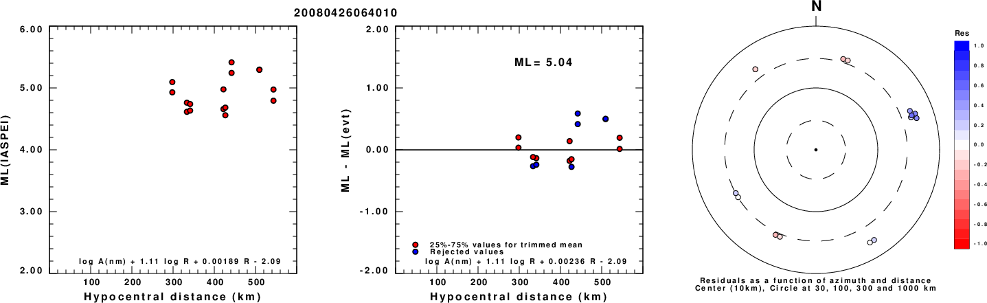
Left: ML computed using the IASPEI formula for Horizontal components. Center: ML residuals computed using a modified IASPEI formula that accounts for path specific attenuation; the values used for the trimmed mean are indicated. The ML relation used for each figure is given at the bottom of each plot.
Right: Residuals from new relation as a function of distance and azimuth.
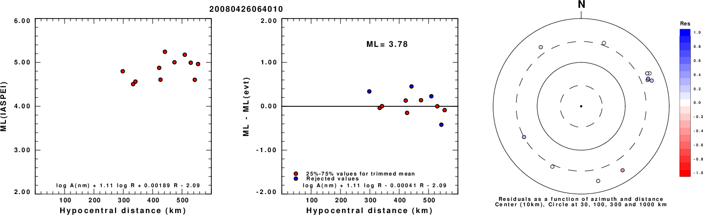
Left: ML computed using the IASPEI formula for Vertical components (research). Center: ML residuals computed using a modified IASPEI formula that accounts for path specific attenuation; the values used for the trimmed mean are indicated. The ML relation used for each figure is given at the bottom of each plot.
Right: Residuals from new relation as a function of distance and azimuth.
Context
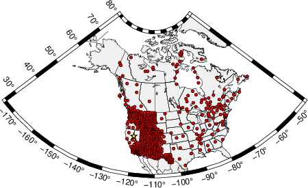
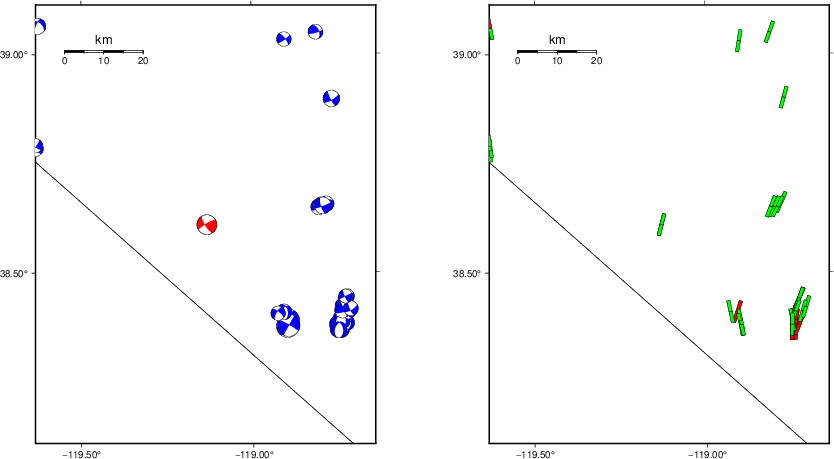
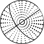
The left panel of the next figure presents the focal mechanism for this earthquake (red) in the context of other nearby events (blue) in the SLU Moment Tensor Catalog. The right panel shows the inferred direction of maximum compressive stress and the type of faulting (green is strike-slip, red is normal, blue is thrust; oblique is shown by a combination of colors). Thus context plot is useful for assessing the appropriateness of the moment tensor of this event.
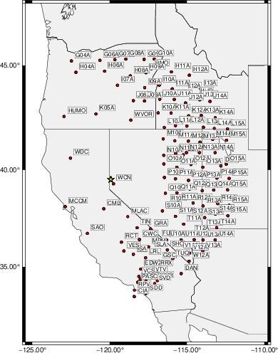
Waveform Inversion using wvfgrd96
The focal mechanism was determined using broadband seismic waveforms. The location of the event (star) and the
stations used for (red) the waveform inversion are shown in the next figure.
|
|
Location of broadband stations used for waveform inversion
|
The program wvfgrd96 was used with good traces observed at short distance to determine the focal mechanism, depth and seismic moment. This technique requires a high quality signal and well determined velocity model for the Green's functions. To the extent that these are the quality data, this type of mechanism should be preferred over the radiation pattern technique which requires the separate step of defining the pressure and tension quadrants and the correct strike.
The observed and predicted traces are filtered using the following gsac commands:
cut o DIST/3.3 -40 o DIST/3.3 +50
rtr
taper w 0.1
hp c 0.03 n 3
lp c 0.07 n 3
The results of this grid search are as follow:
           DEPTH  STK   DIP  RAKE   MW    FIT
WVFGRD96    0.5    55    70     5   4.60 0.4667
WVFGRD96    1.0    55    80     5   4.62 0.5012
WVFGRD96    2.0    55    75     0   4.72 0.6135
WVFGRD96    3.0   235    90    15   4.77 0.6644
WVFGRD96    4.0   235    90    15   4.80 0.6922
WVFGRD96    5.0   235    90    10   4.83 0.7053
WVFGRD96    6.0   240    85    15   4.85 0.7121
WVFGRD96    7.0   240    85    15   4.88 0.7161
WVFGRD96    8.0   240    80    15   4.91 0.7202
WVFGRD96    9.0    60    90   -15   4.92 0.7119
WVFGRD96   10.0   240    85    15   4.93 0.7103
WVFGRD96   11.0   240    85    15   4.95 0.7059
WVFGRD96   12.0   240    85    15   4.96 0.7003
WVFGRD96   13.0   240    85    15   4.97 0.6925
WVFGRD96   14.0   240    80    10   4.98 0.6863
WVFGRD96   15.0   240    80    10   4.99 0.6796
WVFGRD96   16.0   235    90   -10   5.00 0.6706
WVFGRD96   17.0    55    85    10   5.01 0.6694
WVFGRD96   18.0    55    85    10   5.02 0.6620
WVFGRD96   19.0    55    85    10   5.03 0.6532
WVFGRD96   20.0    55    85    10   5.03 0.6442
WVFGRD96   21.0    55    85    10   5.04 0.6329
WVFGRD96   22.0    55    85    10   5.05 0.6223
WVFGRD96   23.0    55    85    10   5.05 0.6101
WVFGRD96   24.0    55    80    10   5.06 0.5986
WVFGRD96   25.0    55    80    10   5.06 0.5865
WVFGRD96   26.0    55    80    10   5.07 0.5737
WVFGRD96   27.0    55    80    10   5.07 0.5629
WVFGRD96   28.0    55    80    10   5.08 0.5515
WVFGRD96   29.0    55    80    10   5.09 0.5404
The best solution is
WVFGRD96 8.0 240 80 15 4.91 0.7202
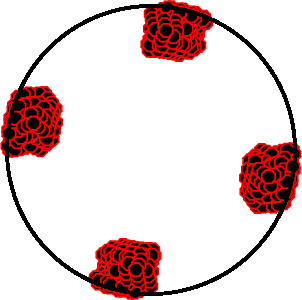
The mechanism corresponding to the best fit is
|
|
Figure 1. Waveform inversion focal mechanism
|
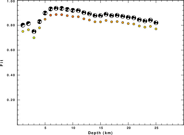
The best fit as a function of depth is given in the following figure:
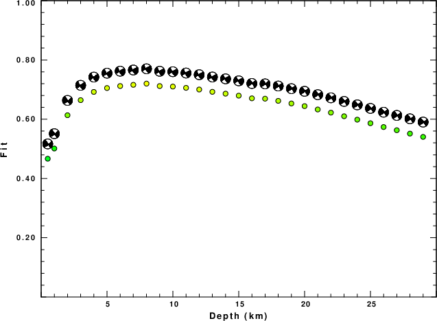
|
|
Figure 2. Depth sensitivity for waveform mechanism
|
The comparison of the observed and predicted waveforms is given in the next figure. The red traces are the observed and the blue are the predicted.
Each observed-predicted component is plotted to the same scale and peak amplitudes are indicated by the numbers to the left of each trace. A pair of numbers is given in black at the right of each predicted traces. The upper number it the time shift required for maximum correlation between the observed and predicted traces. This time shift is required because the synthetics are not computed at exactly the same distance as the observed, the velocity model used in the predictions may not be perfect and the epicentral parameters may be be off.
A positive time shift indicates that the prediction is too fast and should be delayed to match the observed trace (shift to the right in this figure). A negative value indicates that the prediction is too slow. The lower number gives the percentage of variance reduction to characterize the individual goodness of fit (100% indicates a perfect fit).
The bandpass filter used in the processing and for the display was
cut o DIST/3.3 -40 o DIST/3.3 +50
rtr
taper w 0.1
hp c 0.03 n 3
lp c 0.07 n 3

|
|
Figure 3. Waveform comparison for selected depth. Red: observed; Blue - predicted. The time shift with respect to the model prediction is indicated. The percent of fit is also indicated. The time scale is relative to the first trace sample.
|
|
|
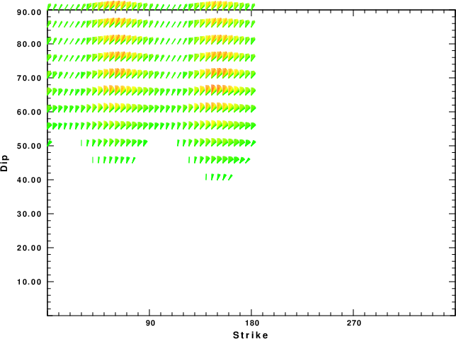
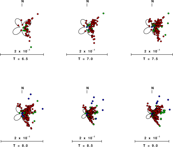
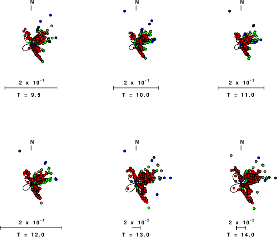
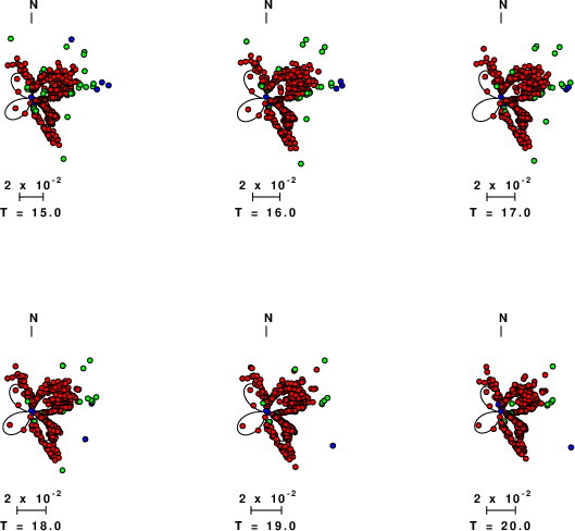
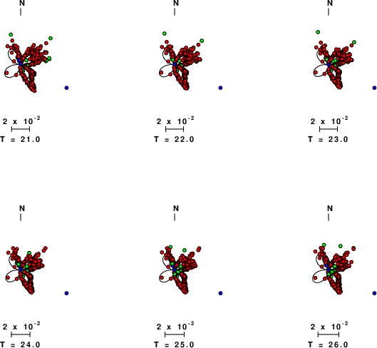
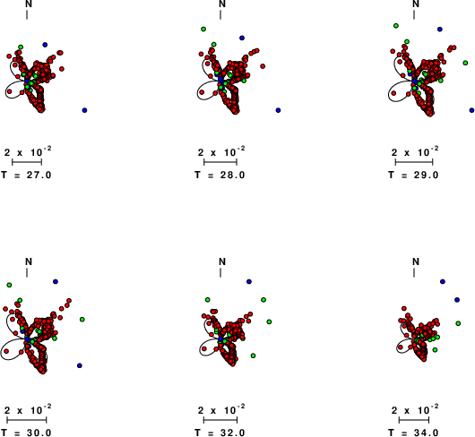
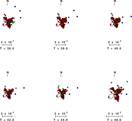
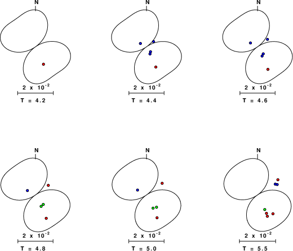
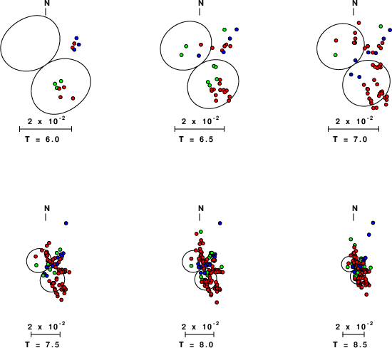
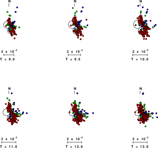
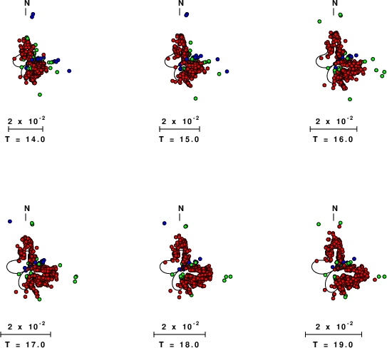
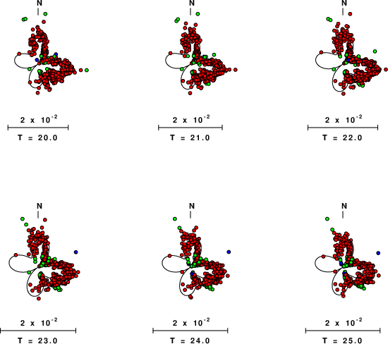
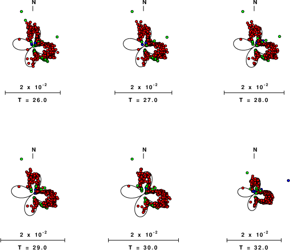
Focal mechanism sensitivity at the preferred depth. The red color indicates a very good fit to the waveforms.
Each solution is plotted as a vector at a given value of strike and dip with the angle of the vector representing the rake angle, measured, with respect to the upward vertical (N) in the figure.
|
A check on the assumed source location is possible by looking at the time shifts between the observed and predicted traces. The time shifts for waveform matching arise for several reasons:
- The origin time and epicentral distance are incorrect
- The velocity model used for the inversion is incorrect
- The velocity model used to define the P-arrival time is not the
same as the velocity model used for the waveform inversion
(assuming that the initial trace alignment is based on the
P arrival time)
Assuming only a mislocation, the time shifts are fit to a functional form:
Time_shift = A + B cos Azimuth + C Sin Azimuth
The time shifts for this inversion lead to the next figure:
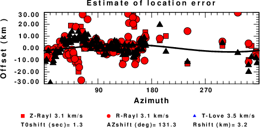
The derived shift in origin time and epicentral coordinates are given at the bottom of the figure.
Surface-Wave Focal Mechanism
The following figure shows the stations used in the grid search for the best focal mechanism to fit the surface-wave spectral amplitudes of the Love and Rayleigh waves.
|
|
Location of broadband stations used to obtain focal mechanism from surface-wave spectral amplitudes
|
The surface-wave determined focal mechanism is shown here.
  NODAL PLANES


  STK=     234.99
  DIP=      90.00
 RAKE=      24.99

             OR

  STK=     144.99
  DIP=      65.01
 RAKE=     179.99


DEPTH = 7.0 km

Mw = 4.95
Best Fit 0.8857 - P-T axis plot gives solutions with FIT greater than FIT90
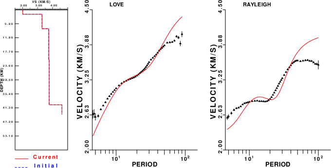
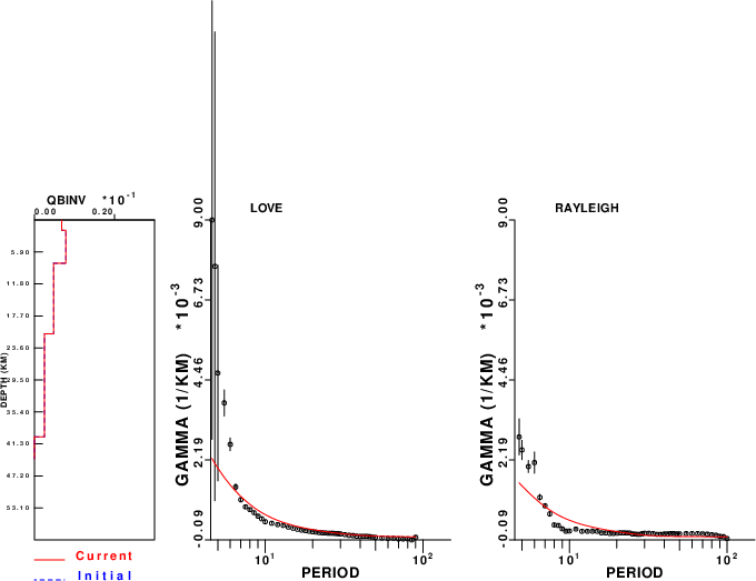
Surface-wave analysis
Surface wave analysis was performed using codes from
Computer Programs in Seismology, specifically the
multiple filter analysis program do_mft and the surface-wave
radiation pattern search program srfgrd96.
Data preparation
Digital data were collected, instrument response removed and traces converted
to Z, R an T components. Multiple filter analysis was applied to the Z and T traces to obtain the Rayleigh- and Love-wave spectral amplitudes, respectively.
These were input to the search program which examined all depths between 1 and 25 km
and all possible mechanisms.
|
|
Best mechanism fit as a function of depth. The preferred depth is given above. Lower hemisphere projection
|
|
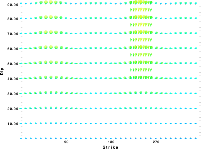
|
Pressure-tension axis trends. Since the surface-wave spectra search does not distinguish between P and T axes and since there is a 180 ambiguity in strike, all possible P and T axes are plotted. First motion data and waveforms will be used to select the preferred mechanism. The purpose of this plot is to provide an idea of the
possible range of solutions. The P and T-axes for all mechanisms with goodness of fit greater than 0.9 FITMAX (above) are plotted here.
|
|
|
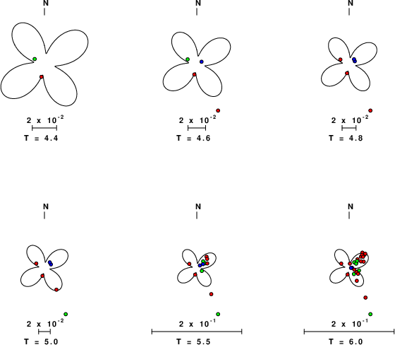
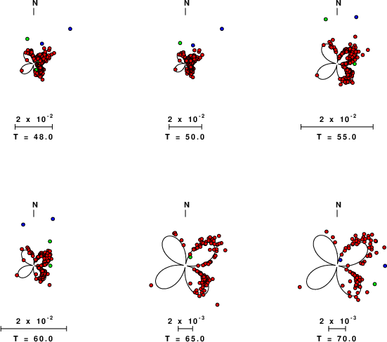
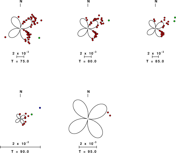
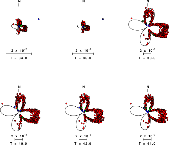
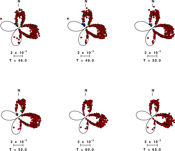
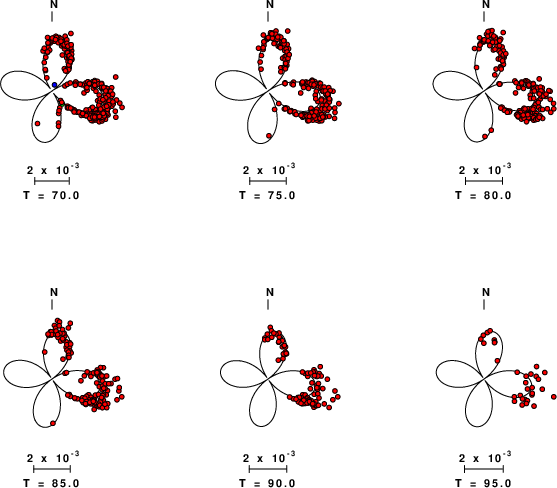
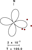
Focal mechanism sensitivity at the preferred depth. The red color indicates a very good fit to the Love and Rayleigh wave radiation patterns.
Each solution is plotted as a vector at a given value of strike and dip with the angle of the vector representing the rake angle, measured, with respect to the upward vertical (N) in the figure. Because of the symmetry of the spectral amplitude rediation patterns, only strikes from 0-180 degrees are sampled.
|
Love-wave radiation patterns
Rayleigh-wave radiation patterns
- Rayleigh-wave radiation patterns.
- Rayleigh-wave radiation patterns.
- Rayleigh-wave radiation patterns.
- Rayleigh-wave radiation patterns.
- Rayleigh-wave radiation patterns.
- Rayleigh-wave radiation patterns.
- Rayleigh-wave radiation patterns.
- Rayleigh-wave radiation patterns.
- Rayleigh-wave radiation patterns.
- Rayleigh-wave radiation patterns.
Waveform comparison for this mechanism
Since the analysis of the surface-wave radiation patterns uses only spectral
amplitudes and because the surfave-wave radiation patterns have a 180 degree symmetry, each surface-wave solution consists of four possible focal mechanisms corresponding to the interchange of the P- and T-axes and a roation of the mechanism by 180 degrees. To select one mechanism, P-wave first motion can be used. This was not possible in this case because all the P-wave first motions were
emergent ( a feature of the P-wave wave takeoff angle, the station location and the mechanism). The other way to select among the mechanisms is to compute
forward synthetics and compare the observed and predicted waveforms.
The fits to the waveforms with the given mechanism are show below:
This figure shows the fit to the three components of motion (Z - vertical, R-radial and T - transverse). For each station and component, the
observed traces is shown in red and the model predicted trace in blue. The traces represent filtered ground velocity in units of meters/sec (the peak value is printed adjacent to each trace; each pair of traces to plotted to the same scale to emphasize the difference in levels). Both synthetic and observed traces have been filtered using the SAC commands:
Appendix A
Spectra fit plots to each station
Velocity Model
The WUS.model used for the waveform synthetic seismograms and for the surface wave eigenfunctions and dispersion is as follows
(The format is in the model96 format of Computer Programs in Seismology).
MODEL.01
Model after     8 iterations
ISOTROPIC
KGS
FLAT EARTH
1-D
CONSTANT VELOCITY
LINE08
LINE09
LINE10
LINE11
      H(KM)   VP(KM/S)   VS(KM/S) RHO(GM/CC)         QP         QS       ETAP       ETAS      FREFP      FREFS
     1.9000     3.4065     2.0089     2.2150  0.302E-02  0.679E-02   0.00       0.00       1.00       1.00
     6.1000     5.5445     3.2953     2.6089  0.349E-02  0.784E-02   0.00       0.00       1.00       1.00
    13.0000     6.2708     3.7396     2.7812  0.212E-02  0.476E-02   0.00       0.00       1.00       1.00
    19.0000     6.4075     3.7680     2.8223  0.111E-02  0.249E-02   0.00       0.00       1.00       1.00
     0.0000     7.9000     4.6200     3.2760  0.164E-10  0.370E-10   0.00       0.00       1.00       1.00
Last Changed Sun Apr 28 01:01:53 PM CDT 2024
