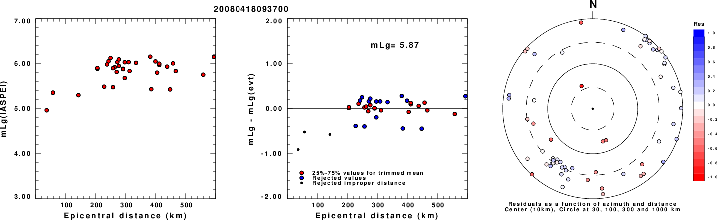
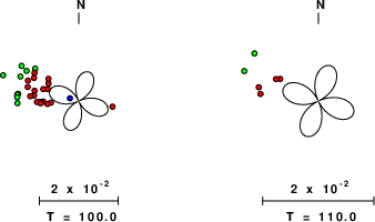
Left: mLg computed using the IASPEI formula. Center: mLg residuals versus epicentral distance ; the values used for the trimmed mean magnitude estimate are indicated. Right: residuals as a function of distance and azimuth.
The ANSS event ID is nm606657 and the event page is at https://earthquake.usgs.gov/earthquakes/eventpage/nm606657/executive.
2008/04/18 09:37:00 38.4515 -87.8862 14.3 5.2 Illinois
 USGS/SLU Moment Tensor Solution
 ENS  2008/04/18 09:37:00:0  38.45  -87.89  14.3 5.2 Illinois

 Best Fitting Double Couple
  Mo = 9.12e+23 dyne-cm
  Mw = 5.24
  Z  = 15 km
  Plane   Strike  Dip  Rake
   NP1       25    90   -175
   NP2      295    85     0
  Principal Axes:
   Axis    Value   Plunge  Azimuth
    T   9.12e+23      4     160
    N   0.00e+00     85      25
    P  -9.12e+23      4     250

 Moment Tensor: (dyne-cm)
    Component   Value
       Mxx     6.96e+23
       Mxy    -5.84e+23
       Mxz    -3.36e+22
       Myy    -6.96e+23
       Myz     7.20e+22
       Mzz     0.00e+00


                     ##############
                 ###################---
              #####################-------
             #####################---------
           #######################-----------
          #######################-------------
         --#####################---------------
        --------###############-----------------
        -------------#########------------------
       ------------------####--------------------
       ---------------------#--------------------
       ---------------------#####----------------
       --------------------##########------------
           ---------------##############--------
         P --------------##################-----
           -------------######################-
          -------------#######################
           -----------#######################
             ---------#####################
              -------#####################
                 ---#############   ###
                     ############ T


 Global CMT Convention Moment Tensor:
      R          T          P
  0.00e+00  -3.36e+22  -7.20e+22
 -3.36e+22   6.96e+23   5.84e+23
 -7.20e+22   5.84e+23  -6.96e+23


Details of the solution is found at

http://www.eas.slu.edu/eqc/eqc_mt/MECH.NA/20080418093700/index.html
|
      STK = 295
      DIP = 85
     RAKE = 0
       MW = 5.24
       HS = 15.0
The NDK file is 20080418093700.ndk The waveform inversion is preferred.
The following compares this source inversion to those provided by others. The purpose is to look for major differences and also to note slight differences that might be inherent to the processing procedure. For completeness the USGS/SLU solution is repeated from above.
 USGS/SLU Moment Tensor Solution
 ENS  2008/04/18 09:37:00:0  38.45  -87.89  14.3 5.2 Illinois

 Best Fitting Double Couple
  Mo = 9.12e+23 dyne-cm
  Mw = 5.24
  Z  = 15 km
  Plane   Strike  Dip  Rake
   NP1       25    90   -175
   NP2      295    85     0
  Principal Axes:
   Axis    Value   Plunge  Azimuth
    T   9.12e+23      4     160
    N   0.00e+00     85      25
    P  -9.12e+23      4     250

 Moment Tensor: (dyne-cm)
    Component   Value
       Mxx     6.96e+23
       Mxy    -5.84e+23
       Mxz    -3.36e+22
       Myy    -6.96e+23
       Myz     7.20e+22
       Mzz     0.00e+00


                     ##############
                 ###################---
              #####################-------
             #####################---------
           #######################-----------
          #######################-------------
         --#####################---------------
        --------###############-----------------
        -------------#########------------------
       ------------------####--------------------
       ---------------------#--------------------
       ---------------------#####----------------
       --------------------##########------------
           ---------------##############--------
         P --------------##################-----
           -------------######################-
          -------------#######################
           -----------#######################
             ---------#####################
              -------#####################
                 ---#############   ###
                     ############ T


 Global CMT Convention Moment Tensor:
      R          T          P
  0.00e+00  -3.36e+22  -7.20e+22
 -3.36e+22   6.96e+23   5.84e+23
 -7.20e+22   5.84e+23  -6.96e+23


Details of the solution is found at

http://www.eas.slu.edu/eqc/eqc_mt/MECH.NA/20080418093700/index.html
|
USGS Body-Wave Moment Tensor Solution

 08/04/18 09:36:57.31
 ILLINOIS
 Epicenter:  38.523  -87.884
 MW 5.2

 USGS MOMENT TENSOR SOLUTION
 Depth  18         No. of sta:  7
 Moment Tensor;   Scale 10**16 Nm
   Mrr=-0.41       Mtt= 7.31
   Mpp=-6.91       Mrt=-1.11
   Mrp=-0.54       Mtp= 5.83
  Principal axes:
   T  Val=  9.55  Plg= 7  Azm=160
   N       -0.56      82      347
   P       -9.00       0      250

 Best Double Couple:Mo=9.3*10**16
  NP1:Strike=296 Dip=84 Slip=   4
  NP2:       205     86       174

               #######
          ###############--
        ################-----
      #################--------
    ##################-----------
   ##################-------------
   -----############--------------
  -----------######----------------
  ---------------#-----------------
  ----------------###--------------
  ---------------########----------
    ------------############-------
  P -----------################---
    ----------####################
    ----------###################
      -------##################
        ----##########   ####
          --########## T ##
               #######
|
April 18, 2008, ILLINOIS, MW=5.3

Goran Ekstrom

CENTROID-MOMENT-TENSOR  SOLUTION
GCMT EVENT:     C200804180936A
DATA: II IU MN CU IC G  GE
L.P.BODY WAVES: 74S, 119C, T= 40
SURFACE WAVES: 103S, 186C, T= 50
TIMESTAMP:      Q-20080418094937
CENTROID LOCATION:
ORIGIN TIME:      09:37:02.2 0.1
LAT:38.55N 0.01;LON: 87.91W 0.01
DEP: 15.0  FIX;TRIANG HDUR:  1.2
MOMENT TENSOR: SCALE 10**24 D-CM
RR=-0.011 0.021; TT= 0.983 0.019
PP=-0.972 0.021; RT= 0.067 0.057
RP=-0.154 0.062; TP= 0.736 0.017
PRINCIPAL AXES:
1.(T) VAL=  1.229;PLG= 1;AZM=342
2.(N)       0.012;    82;     77
3.(P)      -1.241;     8;    251
BEST DBLE.COUPLE:M0= 1.24*10**24
NP1: STRIKE= 27;DIP=84;SLIP=-175
NP2: STRIKE=296;DIP=85;SLIP=  -6

            T #########
        ###   ###########--
      ##################-----
    ###################--------
   ####################---------
  ---#################-----------
  --------###########------------
 -------------######--------------
 -----------------#---------------
 -----------------####------------
    -------------########---------
  P ------------############-----
    -----------################--
   -----------##################
    ---------##################
      ------#################
        ---################
            ###########
|
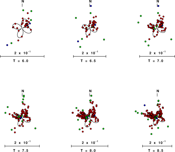
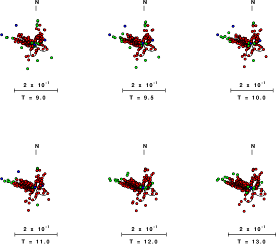
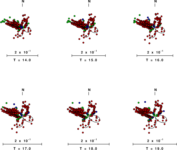
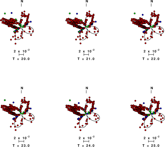
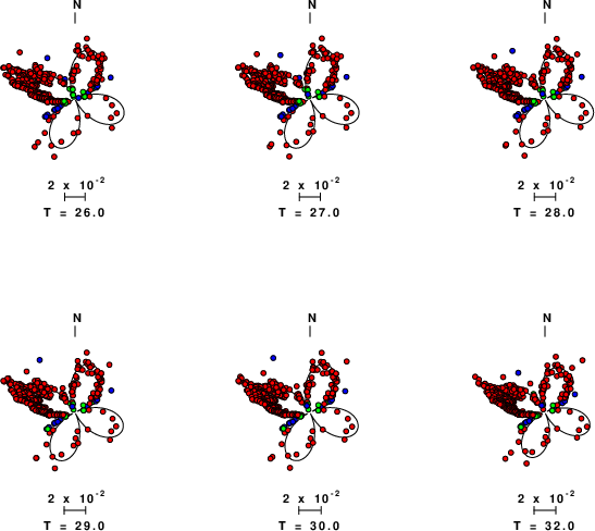
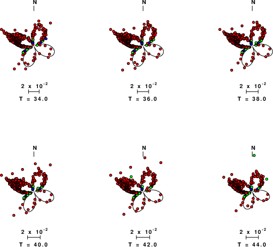
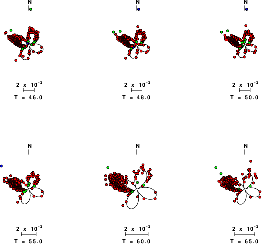
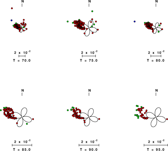
Given the availability of digital waveforms for determination of the moment tensor, this section documents the added processing leading to mLg, if appropriate to the region, and ML by application of the respective IASPEI formulae. As a research study, the linear distance term of the IASPEI formula for ML is adjusted to remove a linear distance trend in residuals to give a regionally defined ML. The defined ML uses horizontal component recordings, but the same procedure is applied to the vertical components since there may be some interest in vertical component ground motions. Residual plots versus distance may indicate interesting features of ground motion scaling in some distance ranges. A residual plot of the regionalized magnitude is given as a function of distance and azimuth, since data sets may transcend different wave propagation provinces.
Left: mLg computed using the IASPEI formula. Center: mLg residuals versus epicentral distance ; the values used for the trimmed mean magnitude estimate are indicated.
Right: residuals as a function of distance and azimuth.
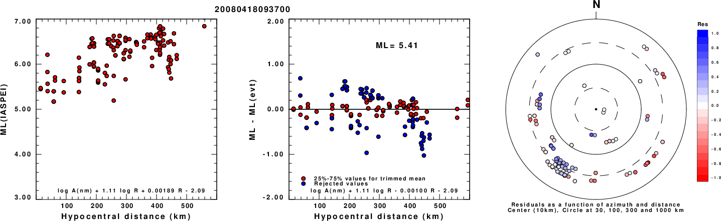
Left: ML computed using the IASPEI formula for Horizontal components. Center: ML residuals computed using a modified IASPEI formula that accounts for path specific attenuation; the values used for the trimmed mean are indicated. The ML relation used for each figure is given at the bottom of each plot.
Right: Residuals from new relation as a function of distance and azimuth.
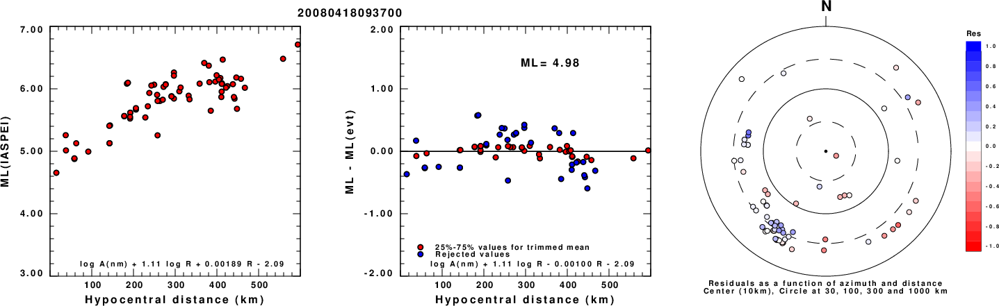
Left: ML computed using the IASPEI formula for Vertical components (research). Center: ML residuals computed using a modified IASPEI formula that accounts for path specific attenuation; the values used for the trimmed mean are indicated. The ML relation used for each figure is given at the bottom of each plot.
Right: Residuals from new relation as a function of distance and azimuth.
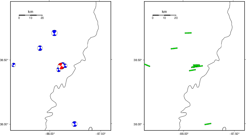 |
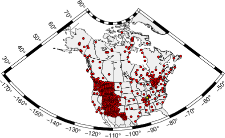
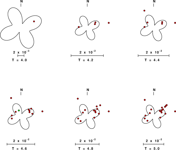
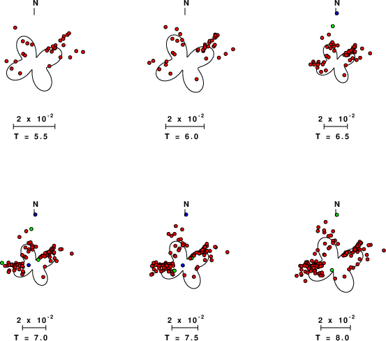
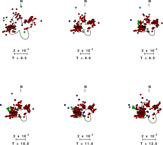
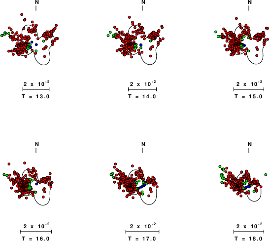
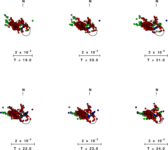
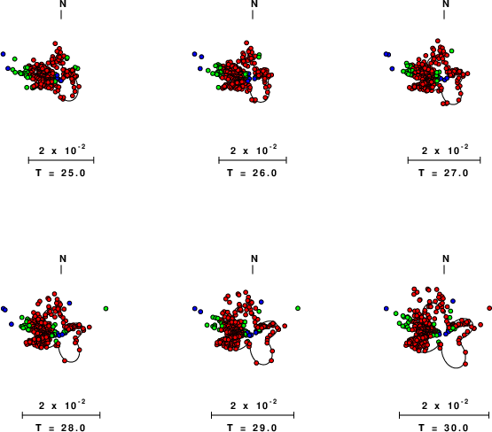
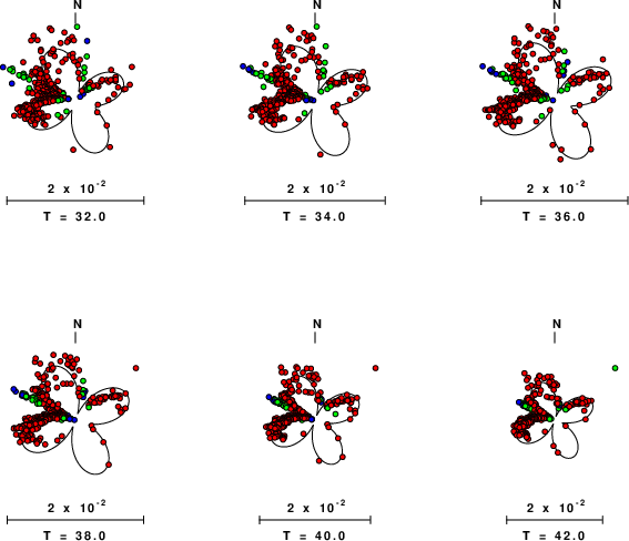
The following figure shows the stations used in the grid search for the best focal mechanism to fit the surface-wave spectral amplitudes of the Love and Rayleigh waves.
|
|
|
The surface-wave determined focal mechanism is shown here.
NODAL PLANES
STK= 199.11
DIP= 85.08
RAKE= 169.97
OR
STK= 289.98
DIP= 80.00
RAKE= 5.00
DEPTH = 15.0 km
Mw = 5.32
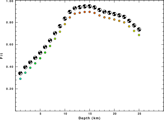
Best Fit 0.8952 - P-T axis plot gives solutions with FIT greater than FIT90
 |
Surface wave analysis was performed using codes from Computer Programs in Seismology, specifically the multiple filter analysis program do_mft and the surface-wave radiation pattern search program srfgrd96.
Digital data were collected, instrument response removed and traces converted
to Z, R an T components. Multiple filter analysis was applied to the Z and T traces to obtain the Rayleigh- and Love-wave spectral amplitudes, respectively.
These were input to the search program which examined all depths between 1 and 25 km
and all possible mechanisms.
|
|
|
|
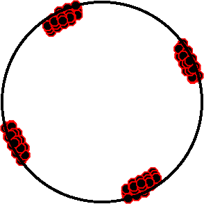
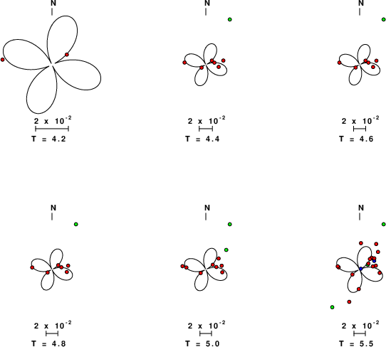
| Pressure-tension axis trends. Since the surface-wave spectra search does not distinguish between P and T axes and since there is a 180 ambiguity in strike, all possible P and T axes are plotted. First motion data and waveforms will be used to select the preferred mechanism. The purpose of this plot is to provide an idea of the possible range of solutions. The P and T-axes for all mechanisms with goodness of fit greater than 0.9 FITMAX (above) are plotted here. |
|
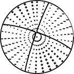
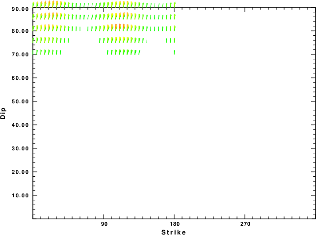
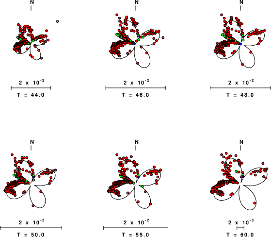
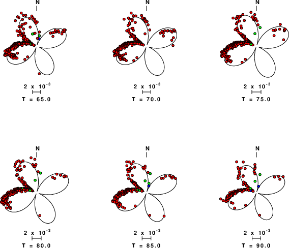
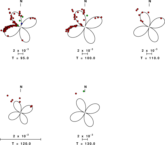
| Focal mechanism sensitivity at the preferred depth. The red color indicates a very good fit to the Love and Rayleigh wave radiation patterns. Each solution is plotted as a vector at a given value of strike and dip with the angle of the vector representing the rake angle, measured, with respect to the upward vertical (N) in the figure. Because of the symmetry of the spectral amplitude rediation patterns, only strikes from 0-180 degrees are sampled. |
|
|
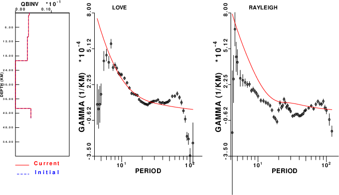
The CUS model used for the waveform synthetic seismograms and for the surface wave eigenfunctions and dispersion is as follows (The format is in the model96 format of Computer Programs in Seismology).
MODEL.01
CUS Model with Q from simple gamma values
ISOTROPIC
KGS
FLAT EARTH
1-D
CONSTANT VELOCITY
LINE08
LINE09
LINE10
LINE11
  H(KM) VP(KM/S) VS(KM/S) RHO(GM/CC)   QP   QS  ETAP  ETAS  FREFP  FREFS
  1.0000  5.0000  2.8900  2.5000 0.172E-02 0.387E-02 0.00  0.00  1.00  1.00
  9.0000  6.1000  3.5200  2.7300 0.160E-02 0.363E-02 0.00  0.00  1.00  1.00
 10.0000  6.4000  3.7000  2.8200 0.149E-02 0.336E-02 0.00  0.00  1.00  1.00
 20.0000  6.7000  3.8700  2.9020 0.000E-04 0.000E-04 0.00  0.00  1.00  1.00
  0.0000  8.1500  4.7000  3.3640 0.194E-02 0.431E-02 0.00  0.00  1.00  1.00