Location
SLU Location
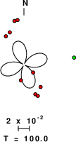
To check the ANSS location or to compare the observed P-wave first motions to the moment tensor solution, P- and S-wave first arrival times were manually read together with the P-wave first motions. The subsequent output of the program elocate is given in the file elocate.txt. The first motion plot is shown below.
Location ANSS
The ANSS event ID is nn00234425 and the event page is at
https://earthquake.usgs.gov/earthquakes/eventpage/nn00234425/executive.
2008/02/21 14:16:05 41.144 -114.872 7.9 5.9 Nevada
Focal Mechanism
 USGS/SLU Moment Tensor Solution
 ENS  2008/02/21 14:16:05:0  41.14 -114.87   7.9 5.9 Nevada

 Stations used:
   IW.DCID1 IW.IMW IW.LOHW IW.MOOW IW.REDW IW.RRI2 IW.SNOW
   IW.TPAW NN.BEK NN.WCN TA.G13A TA.G14A TA.G15A TA.H08A
   TA.H09A TA.H10A TA.H11A TA.H12A TA.H13A TA.H15A TA.H16A
   TA.I08A TA.I09A TA.I11A TA.I12A TA.I13A TA.I14A TA.I15A
   TA.I16A TA.I17A TA.J07A TA.J08A TA.J10A TA.J11A TA.J12A
   TA.J13A TA.J14A TA.J15A TA.J16A TA.J17A TA.J18A TA.K07A
   TA.K08A TA.K09A TA.K10A TA.K12A TA.K13A TA.K14A TA.K15A
   TA.K16A TA.K17A TA.K18A TA.L07A TA.L08A TA.L09A TA.L10A
   TA.L11A TA.L12A TA.L13A TA.L14A TA.L15A TA.L16A TA.L17A
   TA.L18A TA.L19A TA.M07A TA.M09A TA.M10A TA.M11A TA.M13A
   TA.M14A TA.M15A TA.M16A TA.M17A TA.M18A TA.M19A TA.N06A
   TA.N07B TA.N08A TA.N09A TA.N10A TA.N11A TA.N13A TA.N14A
   TA.N15A TA.N16A TA.N17A TA.O06A TA.O07A TA.O08A TA.O09A
   TA.O10A TA.O11A TA.O12A TA.O13A TA.O15A TA.O17A TA.O18A
   TA.O19A TA.P06A TA.P07A TA.P08A TA.P09A TA.P10A TA.P11A
   TA.P12A TA.P14A TA.P15A TA.P16A TA.P17A TA.P18A TA.Q07A
   TA.Q08A TA.Q09A TA.Q10A TA.Q11A TA.Q12A TA.Q13A TA.Q14A
   TA.Q15A TA.Q16A TA.R06C TA.R08A TA.R09A TA.R10A TA.R11A
   TA.R12A TA.R13A TA.R14A TA.R15A TA.R16A TA.R17A TA.S09A
   TA.S10A TA.S11A TA.S12A TA.S13A TA.S14A TA.S15A TA.T11A
   TA.T12A TA.T13A TA.T14A TA.T15A US.AHID US.BMO US.BW06
   US.DUG US.ELK US.HLID US.WVOR UU.SRU

 Filtering commands used:
   hp c 0.01 n 3
   lp c 0.05 n 3

 Best Fitting Double Couple
  Mo = 9.23e+24 dyne-cm
  Mw = 5.91
  Z  = 11 km
  Plane   Strike  Dip  Rake
   NP1      210    50   -90
   NP2       30    40   -90
  Principal Axes:
   Axis    Value   Plunge  Azimuth
    T   9.23e+24      5     300
    N   0.00e+00     -0     210
    P  -9.23e+24     85     120

 Moment Tensor: (dyne-cm)
    Component   Value
       Mxx     2.27e+24
       Mxy    -3.93e+24
       Mxz     8.01e+23
       Myy     6.81e+24
       Myz    -1.39e+24
       Mzz    -9.09e+24


                     ##############
                 ##################----
              ################----------##
             ##############--------------##
            #############----------------####
          T ###########-------------------####
            ##########--------------------#####
        ############----------------------######
        ###########-----------------------######
       ###########------------------------#######
       ##########-----------   -----------#######
       ##########----------- P ----------########
       #########------------   ---------#########
        ########------------------------########
        ########-----------------------#########
         ######----------------------##########
          #####---------------------##########
           #####------------------###########
             ###----------------###########
              ###------------#############
                 -------###############
                     ##############


 Global CMT Convention Moment Tensor:
      R          T          P
 -9.09e+24   8.01e+23   1.39e+24
  8.01e+23   2.27e+24   3.93e+24
  1.39e+24   3.93e+24   6.81e+24


Details of the solution is found at

http://www.eas.slu.edu/eqc/eqc_mt/MECH.NA/20080221141605/index.html
|
Preferred Solution
The preferred solution from an analysis of the surface-wave spectral amplitude radiation pattern, waveform inversion or first motion observations is
      STK = 30
      DIP = 40
     RAKE = -90
       MW = 5.91
       HS = 11.0
The NDK file is 20080221141605.ndk
The waveform inversion is preferred.
Moment Tensor Comparison
The following compares this source inversion to those provided by others. The purpose is to look for major differences and also to note slight differences that might be inherent to the processing procedure. For completeness the USGS/SLU solution is repeated from above.
| SLU |
USGSMT |
CMT |
GCMT |
UCB |
USGSCMT |
SLUFM |
 USGS/SLU Moment Tensor Solution
 ENS  2008/02/21 14:16:05:0  41.14 -114.87   7.9 5.9 Nevada

 Stations used:
   IW.DCID1 IW.IMW IW.LOHW IW.MOOW IW.REDW IW.RRI2 IW.SNOW
   IW.TPAW NN.BEK NN.WCN TA.G13A TA.G14A TA.G15A TA.H08A
   TA.H09A TA.H10A TA.H11A TA.H12A TA.H13A TA.H15A TA.H16A
   TA.I08A TA.I09A TA.I11A TA.I12A TA.I13A TA.I14A TA.I15A
   TA.I16A TA.I17A TA.J07A TA.J08A TA.J10A TA.J11A TA.J12A
   TA.J13A TA.J14A TA.J15A TA.J16A TA.J17A TA.J18A TA.K07A
   TA.K08A TA.K09A TA.K10A TA.K12A TA.K13A TA.K14A TA.K15A
   TA.K16A TA.K17A TA.K18A TA.L07A TA.L08A TA.L09A TA.L10A
   TA.L11A TA.L12A TA.L13A TA.L14A TA.L15A TA.L16A TA.L17A
   TA.L18A TA.L19A TA.M07A TA.M09A TA.M10A TA.M11A TA.M13A
   TA.M14A TA.M15A TA.M16A TA.M17A TA.M18A TA.M19A TA.N06A
   TA.N07B TA.N08A TA.N09A TA.N10A TA.N11A TA.N13A TA.N14A
   TA.N15A TA.N16A TA.N17A TA.O06A TA.O07A TA.O08A TA.O09A
   TA.O10A TA.O11A TA.O12A TA.O13A TA.O15A TA.O17A TA.O18A
   TA.O19A TA.P06A TA.P07A TA.P08A TA.P09A TA.P10A TA.P11A
   TA.P12A TA.P14A TA.P15A TA.P16A TA.P17A TA.P18A TA.Q07A
   TA.Q08A TA.Q09A TA.Q10A TA.Q11A TA.Q12A TA.Q13A TA.Q14A
   TA.Q15A TA.Q16A TA.R06C TA.R08A TA.R09A TA.R10A TA.R11A
   TA.R12A TA.R13A TA.R14A TA.R15A TA.R16A TA.R17A TA.S09A
   TA.S10A TA.S11A TA.S12A TA.S13A TA.S14A TA.S15A TA.T11A
   TA.T12A TA.T13A TA.T14A TA.T15A US.AHID US.BMO US.BW06
   US.DUG US.ELK US.HLID US.WVOR UU.SRU

 Filtering commands used:
   hp c 0.01 n 3
   lp c 0.05 n 3

 Best Fitting Double Couple
  Mo = 9.23e+24 dyne-cm
  Mw = 5.91
  Z  = 11 km
  Plane   Strike  Dip  Rake
   NP1      210    50   -90
   NP2       30    40   -90
  Principal Axes:
   Axis    Value   Plunge  Azimuth
    T   9.23e+24      5     300
    N   0.00e+00     -0     210
    P  -9.23e+24     85     120

 Moment Tensor: (dyne-cm)
    Component   Value
       Mxx     2.27e+24
       Mxy    -3.93e+24
       Mxz     8.01e+23
       Myy     6.81e+24
       Myz    -1.39e+24
       Mzz    -9.09e+24


                     ##############
                 ##################----
              ################----------##
             ##############--------------##
            #############----------------####
          T ###########-------------------####
            ##########--------------------#####
        ############----------------------######
        ###########-----------------------######
       ###########------------------------#######
       ##########-----------   -----------#######
       ##########----------- P ----------########
       #########------------   ---------#########
        ########------------------------########
        ########-----------------------#########
         ######----------------------##########
          #####---------------------##########
           #####------------------###########
             ###----------------###########
              ###------------#############
                 -------###############
                     ##############


 Global CMT Convention Moment Tensor:
      R          T          P
 -9.09e+24   8.01e+23   1.39e+24
  8.01e+23   2.27e+24   3.93e+24
  1.39e+24   3.93e+24   6.81e+24


Details of the solution is found at

http://www.eas.slu.edu/eqc/eqc_mt/MECH.NA/20080221141605/index.html
|
USGS Body-Wave Moment Tensor Solution

 08/02/21 14:16:03.82
 NEVADA
 Epicenter:  41.083 -114.730
 MW 5.8

 USGS MOMENT TENSOR SOLUTION
 Depth   7         No. of sta: 91
 Moment Tensor;   Scale 10**17 Nm
   Mrr=-6.82       Mtt= 2.12
   Mpp= 4.70       Mrt= 1.59
   Mrp= 2.38       Mtp= 1.19
  Principal axes:
   T  Val=  5.79  Plg=12  Azm=293
   N        1.69       3       23
   P       -7.48      76      128

 Best Double Couple:Mo=6.8*10**17
  NP1:Strike=206 Dip=58 Slip= -86
  NP2:        19     33       -96

               #######
          #################
        ##############-----##
      #############---------###
    #############------------####
   #   #########-------------#####
   # T ########---------------####
  ##   #######----------------#####
  ###########-----------------#####
  ##########-------   --------#####
  #########-------- P -------######
  #########--------   -------######
   #######------------------######
   #######-----------------#######
    ######----------------#######
      ####--------------#######
        ##------------#######
          #-------#########
               #######
|
February 21, 2008, NEVADA, MW=6.0

Goran Ekstrom

CENTROID-MOMENT-TENSOR  SOLUTION
GCMT EVENT:     C200802211416A
DATA: II IU CU IC G  GE
L.P.BODY WAVES: 92S, 209C, T= 40
MANTLE WAVES:   83S, 120C, T=125
SURFACE WAVES:  99S, 252C, T= 50
TIMESTAMP:      Q-20080221151936
CENTROID LOCATION:
ORIGIN TIME:      14:16:10.1 0.1
LAT:41.23N 0.01;LON:114.86W 0.01
DEP: 14.1  0.2;TRIANG HDUR:  2.5
MOMENT TENSOR: SCALE 10**25 D-CM
RR=-1.230 0.010; TT= 0.245 0.008
PP= 0.990 0.009; RT=-0.078 0.018
RP= 0.125 0.018; TP= 0.628 0.007
PRINCIPAL AXES:
1.(T) VAL=  1.350;PLG= 2;AZM=300
2.(N)      -0.098;     7;    209
3.(P)      -1.247;    83;     43
BEST DBLE.COUPLE:M0= 1.30*10**25
NP1: STRIKE= 36;DIP=44;SLIP= -81
NP2: STRIKE=203;DIP=47;SLIP= -99

            ###########
        ###########--------
      ##########------------#
     #########--------------###
   T #######-----------------###
     ######------------------####
  ########-------------------####
 ########--------   ---------#####
 ########-------- P --------######
 #######---------   -------#######
 #######-------------------#######
  ######-----------------########
  ######----------------#########
   #####--------------##########
    ####------------###########
      ###--------############
        --#################
            ###########
|
UCB Seismological Laboratory

Inversion method:   complete waveform
Stations used:      CMB KCC ORV

 Berkeley Moment Tensor Solution

 Best Fitting Double-Couple:
    Mo = 1.04E+25 Dyne-cm
    Mw = 5.95
    Z  = 11
    Plane   Strike   Rake   Dip
     NP1      228     -71    65
     NP2       10    -124    31

 Principal Axes:
    Axis    Value   Plunge   Azimuth
      T    10.400      18      305
      N     0.000      17       40
      P   -10.400      65      171

 Event Date/Time: February 21, 2008 at 14:16:05 UTC
 Event ID:        usus2008nsa9
 Moment Tensor: Scale = 10**24 Dyne-cm
    Component   Value
       Mxx      1.254
       Mxy     -4.116
       Mxz      5.612
       Myy      6.359
       Myz     -3.121
       Mzz     -7.613


                    #######
              ################---
           #####################----
         ########################-----
       ###########################-#####
      ##   ###################-----######
     ### T ###############----------######
    ####   ############-------------#######
    #################----------------######
   ################------------------#######
   ##############--------------------#######
   ############----------------------#######
   ###########-----------------------#######
   ##########----------   -----------#######
    #######------------ P ----------#######
    ######-------------   ---------########
     #####------------------------########
      ###------------------------########
       #------------------------########
         ---------------------########
           -----------------########
              -----------########
                    #######

     Lower Hemisphere Equiangle Projection
|
USGS Centroid Moment Tensor Solution

 08/02/21 14:16:03.82
 NEVADA
 Epicenter:  41.083 -114.730
 MW 6.0

 USGS CENTROID MOMENT TENSOR
 08/02/21 14:16:41.29
 Centroid:   42.125 -113.949
 Depth  10         No. of sta: 60
 Moment Tensor;   Scale 10**18 Nm
   Mrr=-1.12       Mtt= 0.26
   Mpp= 0.85       Mrt= 0.29
   Mrp=-0.60       Mtp= 0.53
  Principal axes:
   T  Val=  1.23  Plg= 9  Azm=116
   N        0.16      20       22
   P       -1.40      66      229

 Best Double Couple:Mo=1.3*10**18
  NP1:Strike=  9 Dip=58 Slip=-114
  NP2:       230     40       -55

               ######-
          ############-----
        ###############------
      #############-----#######
    ###########---------#########
   ##########------------#########
   ########--------------#########
  #######----------------##########
  ######-----------------##########
  #####------------------##########
  ####--------   -------###########
  ####-------- P -------###########
   ##---------   ------########
   ##------------------######## T
    #-----------------#########
      ---------------##########
        ------------#########
          --------#########
               -######
|

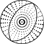
First motions and takeoff angles from an elocate run.
|
Magnitudes
Given the availability of digital waveforms for determination of the moment tensor, this section documents the added processing leading to mLg, if appropriate to the region, and ML by application of the respective IASPEI formulae. As a research study, the linear distance term of the IASPEI formula
for ML is adjusted to remove a linear distance trend in residuals to give a regionally defined ML. The defined ML uses horizontal component recordings, but the same procedure is applied to the vertical components since there may be some interest in vertical component ground motions. Residual plots versus distance may indicate interesting features of ground motion scaling in some distance ranges. A residual plot of the regionalized magnitude is given as a function of distance and azimuth, since data sets may transcend different wave propagation provinces.
ML Magnitude
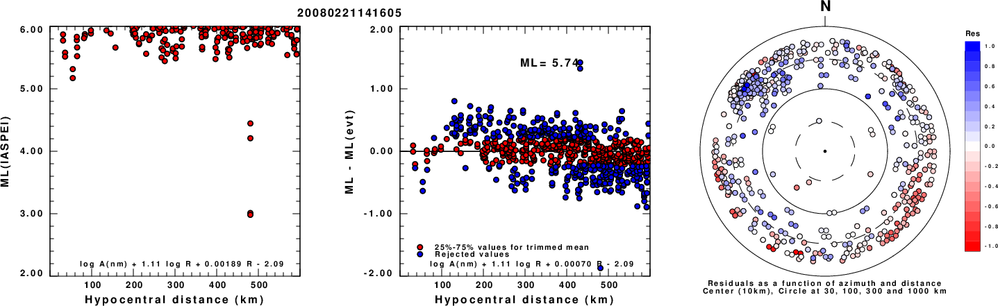
Left: ML computed using the IASPEI formula for Horizontal components. Center: ML residuals computed using a modified IASPEI formula that accounts for path specific attenuation; the values used for the trimmed mean are indicated. The ML relation used for each figure is given at the bottom of each plot.
Right: Residuals from new relation as a function of distance and azimuth.
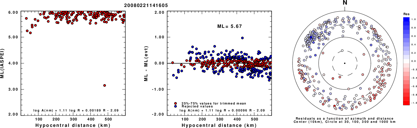
Left: ML computed using the IASPEI formula for Vertical components (research). Center: ML residuals computed using a modified IASPEI formula that accounts for path specific attenuation; the values used for the trimmed mean are indicated. The ML relation used for each figure is given at the bottom of each plot.
Right: Residuals from new relation as a function of distance and azimuth.
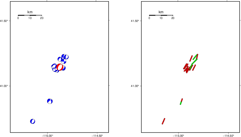
Context
The left panel of the next figure presents the focal mechanism for this earthquake (red) in the context of other nearby events (blue) in the SLU Moment Tensor Catalog. The right panel shows the inferred direction of maximum compressive stress and the type of faulting (green is strike-slip, red is normal, blue is thrust; oblique is shown by a combination of colors). Thus context plot is useful for assessing the appropriateness of the moment tensor of this event.
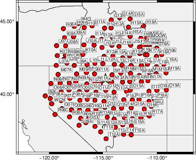
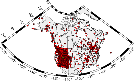
Waveform Inversion using wvfgrd96
The focal mechanism was determined using broadband seismic waveforms. The location of the event (star) and the
stations used for (red) the waveform inversion are shown in the next figure.
|
|
Location of broadband stations used for waveform inversion
|
The program wvfgrd96 was used with good traces observed at short distance to determine the focal mechanism, depth and seismic moment. This technique requires a high quality signal and well determined velocity model for the Green's functions. To the extent that these are the quality data, this type of mechanism should be preferred over the radiation pattern technique which requires the separate step of defining the pressure and tension quadrants and the correct strike.
The observed and predicted traces are filtered using the following gsac commands:
hp c 0.01 n 3
lp c 0.05 n 3
The results of this grid search are as follow:
           DEPTH  STK   DIP  RAKE   MW    FIT
WVFGRD96    0.5    75    90    15   5.47 0.3480
WVFGRD96    1.0   255    90   -10   5.49 0.3692
WVFGRD96    2.0    75    75    -5   5.58 0.4315
WVFGRD96    3.0    70    50   -10   5.67 0.4634
WVFGRD96    4.0    70    45   -15   5.71 0.4994
WVFGRD96    5.0    70    45   -15   5.73 0.5362
WVFGRD96    6.0    65    45   -25   5.75 0.5714
WVFGRD96    7.0    50    40   -55   5.81 0.6128
WVFGRD96    8.0    45    35   -65   5.87 0.6595
WVFGRD96    9.0   205    50   -95   5.90 0.7102
WVFGRD96   10.0    35    40   -80   5.90 0.7386
WVFGRD96   11.0    30    40   -90   5.91 0.7403
WVFGRD96   12.0    35    40   -80   5.90 0.7245
WVFGRD96   13.0    35    40   -80   5.89 0.6981
WVFGRD96   14.0    50    45   -60   5.87 0.6700
WVFGRD96   15.0    65    55   -30   5.84 0.6500
WVFGRD96   16.0    70    60   -20   5.84 0.6350
WVFGRD96   17.0    70    65   -20   5.84 0.6216
WVFGRD96   18.0    70    65   -15   5.85 0.6096
WVFGRD96   19.0    70    65   -15   5.85 0.5972
WVFGRD96   20.0    75    70   -10   5.86 0.5847
WVFGRD96   21.0    75    70   -10   5.86 0.5730
WVFGRD96   22.0    75    70    -5   5.86 0.5602
WVFGRD96   23.0    75    75     5   5.87 0.5488
WVFGRD96   24.0    75    75     5   5.87 0.5372
WVFGRD96   25.0    75    75     5   5.88 0.5253
WVFGRD96   26.0    75    75     5   5.88 0.5131
WVFGRD96   27.0    75    75     5   5.89 0.5012
WVFGRD96   28.0    75    75     5   5.89 0.4894
WVFGRD96   29.0    75    80     5   5.90 0.4782
The best solution is
WVFGRD96 11.0 30 40 -90 5.91 0.7403
The mechanism corresponding to the best fit is
|
|
Figure 1. Waveform inversion focal mechanism
|
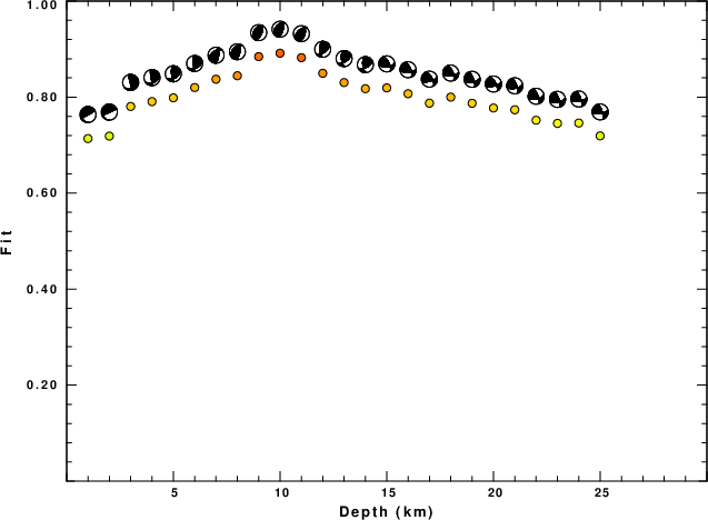
The best fit as a function of depth is given in the following figure:
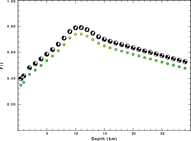
|
|
Figure 2. Depth sensitivity for waveform mechanism
|
The comparison of the observed and predicted waveforms is given in the next figure. The red traces are the observed and the blue are the predicted.
Each observed-predicted component is plotted to the same scale and peak amplitudes are indicated by the numbers to the left of each trace. A pair of numbers is given in black at the right of each predicted traces. The upper number it the time shift required for maximum correlation between the observed and predicted traces. This time shift is required because the synthetics are not computed at exactly the same distance as the observed, the velocity model used in the predictions may not be perfect and the epicentral parameters may be be off.
A positive time shift indicates that the prediction is too fast and should be delayed to match the observed trace (shift to the right in this figure). A negative value indicates that the prediction is too slow. The lower number gives the percentage of variance reduction to characterize the individual goodness of fit (100% indicates a perfect fit).
The bandpass filter used in the processing and for the display was
hp c 0.01 n 3
lp c 0.05 n 3

|
|
Figure 3. Waveform comparison for selected depth. Red: observed; Blue - predicted. The time shift with respect to the model prediction is indicated. The percent of fit is also indicated. The time scale is relative to the first trace sample.
|
|
|
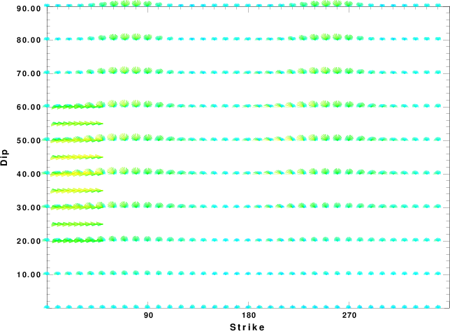
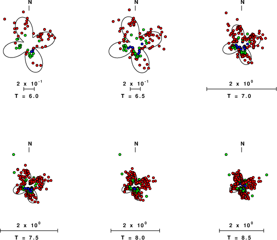
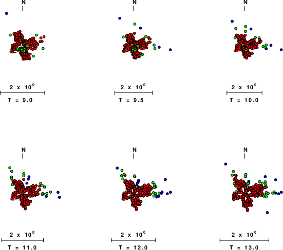
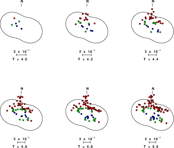
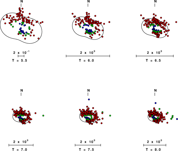
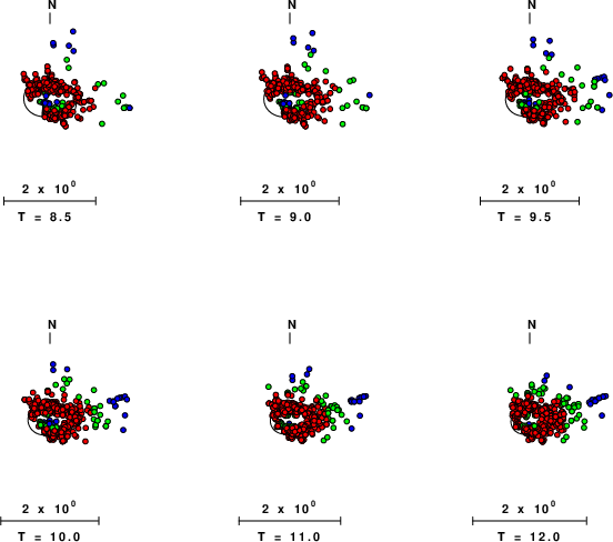
Focal mechanism sensitivity at the preferred depth. The red color indicates a very good fit to the waveforms.
Each solution is plotted as a vector at a given value of strike and dip with the angle of the vector representing the rake angle, measured, with respect to the upward vertical (N) in the figure.
|
A check on the assumed source location is possible by looking at the time shifts between the observed and predicted traces. The time shifts for waveform matching arise for several reasons:
- The origin time and epicentral distance are incorrect
- The velocity model used for the inversion is incorrect
- The velocity model used to define the P-arrival time is not the
same as the velocity model used for the waveform inversion
(assuming that the initial trace alignment is based on the
P arrival time)
Assuming only a mislocation, the time shifts are fit to a functional form:
Time_shift = A + B cos Azimuth + C Sin Azimuth
The time shifts for this inversion lead to the next figure:
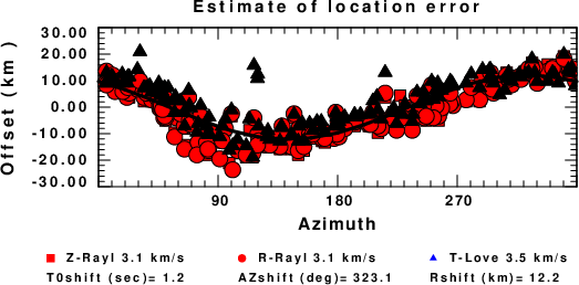
The derived shift in origin time and epicentral coordinates are given at the bottom of the figure.
Surface-Wave Focal Mechanism
The following figure shows the stations used in the grid search for the best focal mechanism to fit the surface-wave spectral amplitudes of the Love and Rayleigh waves.
|
|
Location of broadband stations used to obtain focal mechanism from surface-wave spectral amplitudes
|
The surface-wave determined focal mechanism is shown here.
  NODAL PLANES


  STK=     194.99
  DIP=      55.00
 RAKE=    -104.99

             OR

  STK=      40.01
  DIP=      37.70
 RAKE=     -69.72


DEPTH = 10.0 km

Mw = 5.97
Best Fit 0.8931 - P-T axis plot gives solutions with FIT greater than FIT90
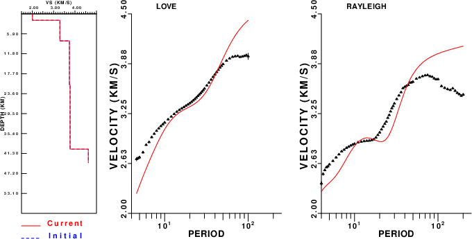
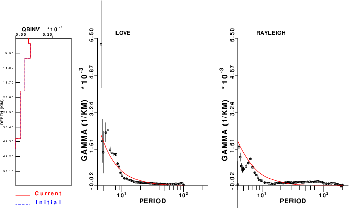
Surface-wave analysis
Surface wave analysis was performed using codes from
Computer Programs in Seismology, specifically the
multiple filter analysis program do_mft and the surface-wave
radiation pattern search program srfgrd96.
Data preparation
Digital data were collected, instrument response removed and traces converted
to Z, R an T components. Multiple filter analysis was applied to the Z and T traces to obtain the Rayleigh- and Love-wave spectral amplitudes, respectively.
These were input to the search program which examined all depths between 1 and 25 km
and all possible mechanisms.
|
|
Best mechanism fit as a function of depth. The preferred depth is given above. Lower hemisphere projection
|
|
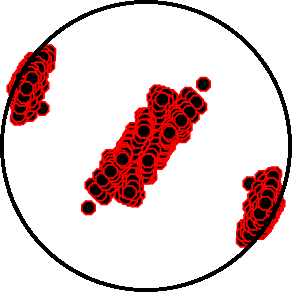
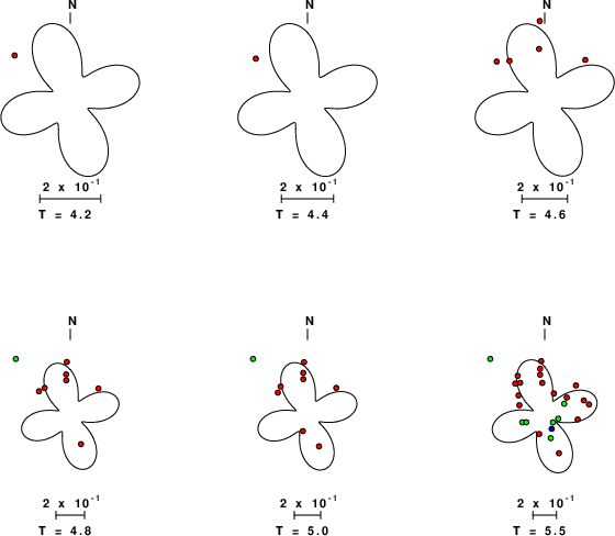
|
Pressure-tension axis trends. Since the surface-wave spectra search does not distinguish between P and T axes and since there is a 180 ambiguity in strike, all possible P and T axes are plotted. First motion data and waveforms will be used to select the preferred mechanism. The purpose of this plot is to provide an idea of the
possible range of solutions. The P and T-axes for all mechanisms with goodness of fit greater than 0.9 FITMAX (above) are plotted here.
|
|
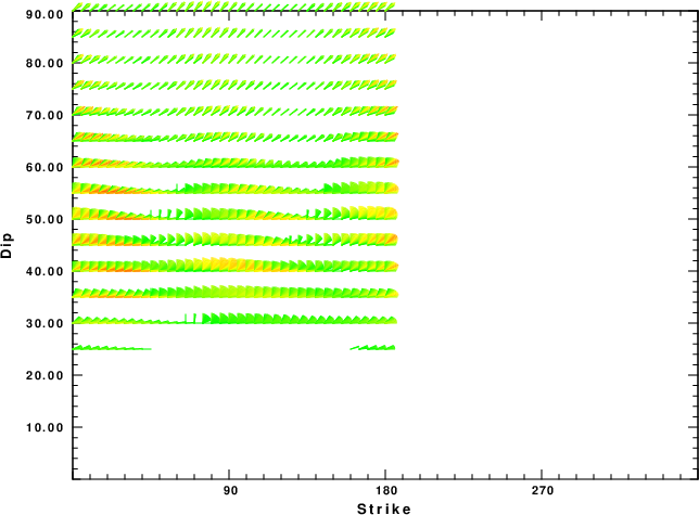
|
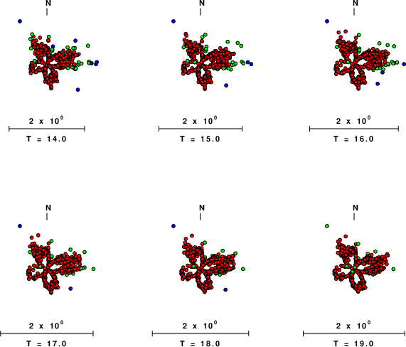
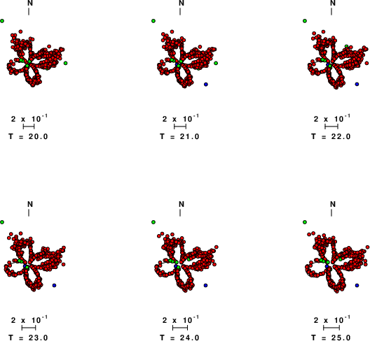
Focal mechanism sensitivity at the preferred depth. The red color indicates a very good fit to the Love and Rayleigh wave radiation patterns.
Each solution is plotted as a vector at a given value of strike and dip with the angle of the vector representing the rake angle, measured, with respect to the upward vertical (N) in the figure. Because of the symmetry of the spectral amplitude rediation patterns, only strikes from 0-180 degrees are sampled.
|
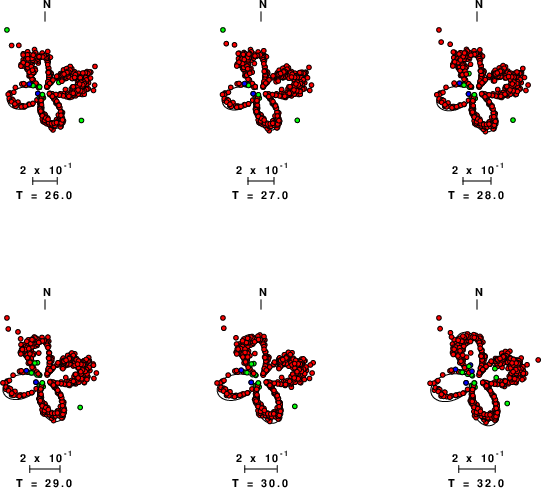
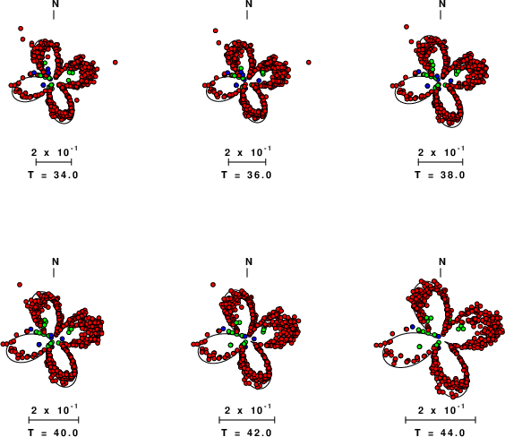
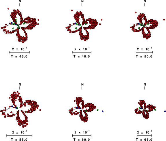
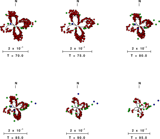
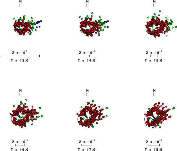
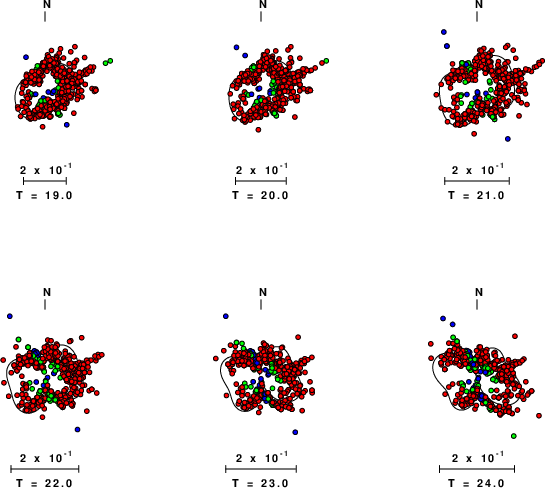
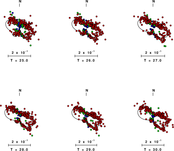
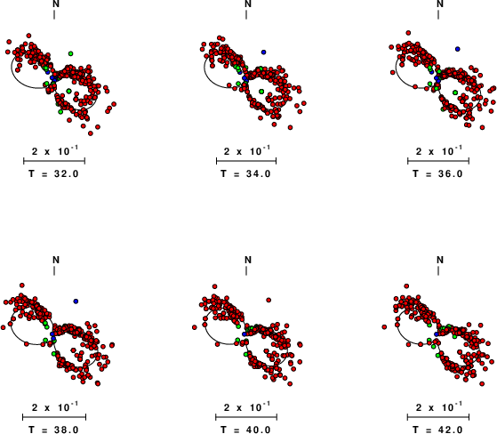
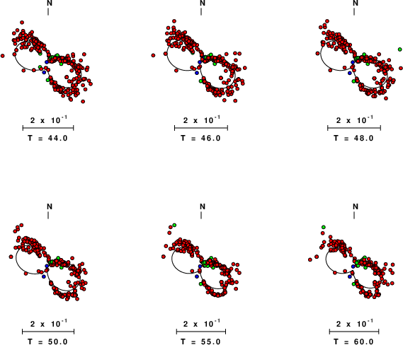
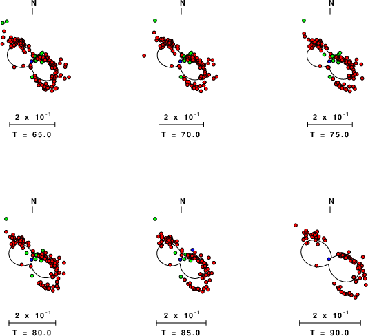
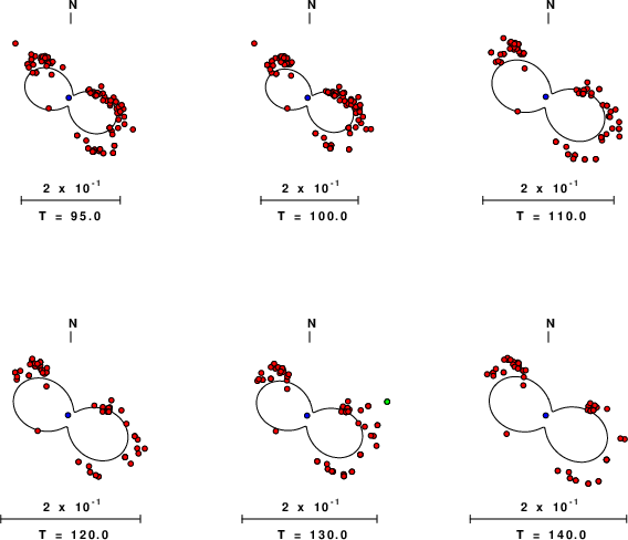
Love-wave radiation patterns
Rayleigh-wave radiation patterns