The ANSS event ID is ci12245763 and the event page is at https://earthquake.usgs.gov/earthquakes/eventpage/ci12245763/executive.
2006/05/24 04:20:27 32.307 -115.228 6.0 5.37 Baja California, Mexico
 USGS/SLU Moment Tensor Solution
 ENS  2006/05/24 04:20:27:0  32.31 -115.23   6.0 5.4 Baja California, Mexico

 Stations used:
   CI.BAR CI.GLA CI.GSC CI.MWC LB.DAC LB.MVU LB.TPH US.ISA
   US.MNV US.TUC

 Filtering commands used:
   cut o DIST/3.3 -30 o DIST/3.3 +90
   rtr
   taper w 0.1
   hp c 0.03 n 3
   lp c 0.05 n 3

 Best Fitting Double Couple
  Mo = 4.90e+23 dyne-cm
  Mw = 5.06
  Z  = 2 km
  Plane   Strike  Dip  Rake
   NP1       36    50   -86
   NP2      210    40   -95
  Principal Axes:
   Axis    Value   Plunge  Azimuth
    T   4.90e+23      5     124
    N   0.00e+00      3     214
    P  -4.90e+23     84     336

 Moment Tensor: (dyne-cm)
    Component   Value
       Mxx     1.44e+23
       Mxy    -2.22e+23
       Mxz    -7.07e+22
       Myy     3.37e+23
       Myz     5.70e+22
       Mzz    -4.81e+23


                     ##############
                 ###############-------
              #############--------------#
             ###########-----------------##
           ###########--------------------###
          ##########----------------------####
         ##########-----------------------#####
        #########------------------------#######
        ########-------------------------#######
       #########----------   ------------########
       ########----------- P -----------#########
       #######------------   ----------##########
       #######------------------------###########
        ######-----------------------###########
        ######----------------------############
         #####--------------------#########   #
          ####------------------########### T
           ####---------------#############
             ##------------################
              ##-------###################
                 ######################
                     ##############


 Global CMT Convention Moment Tensor:
      R          T          P
 -4.81e+23  -7.07e+22  -5.70e+22
 -7.07e+22   1.44e+23   2.22e+23
 -5.70e+22   2.22e+23   3.37e+23


Details of the solution is found at

http://www.eas.slu.edu/eqc/eqc_mt/MECH.NA/20060524042027/index.html
|
      STK = 210
      DIP = 40
     RAKE = -95
       MW = 5.06
       HS = 2.0
The NDK file is 20060524042027.ndk The waveform inversion is preferred.
The following compares this source inversion to those provided by others. The purpose is to look for major differences and also to note slight differences that might be inherent to the processing procedure. For completeness the USGS/SLU solution is repeated from above.
 USGS/SLU Moment Tensor Solution
 ENS  2006/05/24 04:20:27:0  32.31 -115.23   6.0 5.4 Baja California, Mexico

 Stations used:
   CI.BAR CI.GLA CI.GSC CI.MWC LB.DAC LB.MVU LB.TPH US.ISA
   US.MNV US.TUC

 Filtering commands used:
   cut o DIST/3.3 -30 o DIST/3.3 +90
   rtr
   taper w 0.1
   hp c 0.03 n 3
   lp c 0.05 n 3

 Best Fitting Double Couple
  Mo = 4.90e+23 dyne-cm
  Mw = 5.06
  Z  = 2 km
  Plane   Strike  Dip  Rake
   NP1       36    50   -86
   NP2      210    40   -95
  Principal Axes:
   Axis    Value   Plunge  Azimuth
    T   4.90e+23      5     124
    N   0.00e+00      3     214
    P  -4.90e+23     84     336

 Moment Tensor: (dyne-cm)
    Component   Value
       Mxx     1.44e+23
       Mxy    -2.22e+23
       Mxz    -7.07e+22
       Myy     3.37e+23
       Myz     5.70e+22
       Mzz    -4.81e+23


                     ##############
                 ###############-------
              #############--------------#
             ###########-----------------##
           ###########--------------------###
          ##########----------------------####
         ##########-----------------------#####
        #########------------------------#######
        ########-------------------------#######
       #########----------   ------------########
       ########----------- P -----------#########
       #######------------   ----------##########
       #######------------------------###########
        ######-----------------------###########
        ######----------------------############
         #####--------------------#########   #
          ####------------------########### T
           ####---------------#############
             ##------------################
              ##-------###################
                 ######################
                     ##############


 Global CMT Convention Moment Tensor:
      R          T          P
 -4.81e+23  -7.07e+22  -5.70e+22
 -7.07e+22   1.44e+23   2.22e+23
 -5.70e+22   2.22e+23   3.37e+23


Details of the solution is found at

http://www.eas.slu.edu/eqc/eqc_mt/MECH.NA/20060524042027/index.html
|
** SCSN Moment Tensor Solution Message **

REAL-TIME SOLUTION: OPERATOR REVIEWED
Reviewed On: 05/24/2006 17:46:8

Inversion Method: Complete Waveform
Number of Stations used: 6
Stations: CI.IRM CI.BAR CI.DVT AZ.YAQ CI.SWS CI.RXH

Real-Time Solution:
-------------------
Event ID    : 12245763
Magnitude   : 5.16
Depth (km)  : 6.0
Origin Time :  05/24/2006 04:20:26:010
Latitude    : 32.31
Longitude   : -115.23
Further Information at: http://pasadena.wr.usgs.gov/recenteqs/Quakes/ci12245763.htm

SCSN Moment Tensor Solution:
----------------------------
Moment Magnitude     : 5.37
Depth (km)           : 5
Variance Reduction(%): 81.12
Quality Factor       : A
   (A : Mw, MT good enough for distribution)
   (B : Mw only good enough for distribution)
   (C : Solution needs review before distribution)


Best Fitting Double Couple and CLVD Solution:
---------------------------------------------------

Moment Tensor: Scale = 10**21 Dyne-cm
    Component   Value
       Mxx      436
       Mxy      -487
       Mxz      67.1
       Myy      886
       Myz      23.7
       Mzz      -1320

Best Fitting Double Couple Solution:
--------------------------------------------------
 Moment Tensor: Scale = 10**24 Dyne-cm
    Component   Value
       Mxx      0.403
       Mxy     -0.646
       Mxz      0.058
       Myy      1.023
       Myz      0.040
       Mzz     -1.425

 Principle Axes:
    Axis    Value   Plunge   Azimuth
      T     1.429       0      122
      N     0.000       3       32
      P    -1.429      87      214

 Best Fitting Double-Couple:
    Mo = 1.43E+24 Dyne-cm
    Plane   Strike   Rake   Dip
     NP1       29     -94    45
     NP2      215     -86    45

 Moment Magnitude = 5.37


                    #######
              ###################
           ####################---##
         ################----------###
       ###############-------------#####
      ##############----------------#####
     #############------------------######
    ############--------------------#######
    ###########---------------------#######
   ###########----------------------########
   ##########---------   ----------#########
   #########---------- P ----------#########
   ########-----------   ---------##########
   ########----------------------###########
    ######----------------------###########
    ######---------------------############
     #####--------------------#########
      ####------------------########### T
       ###----------------#############
         ##------------###############
           #--------################
              ###################
                    #######

     Lower Hemisphere Equiangle Projection

=============  Station Information ==============

Name       Distance     Azimuth     VR      ZCore
-------------------------------------------------
CI.IRM      205.002      2.188   74.911     24.00
CI.BAR      141.595    287.227   82.649     20.00
CI.DVT       90.517    295.551   84.515     12.00
AZ.YAQ      141.825    312.342   80.599     19.00
CI.SWS       87.807    322.948   79.474     10.00
CI.RXH      103.562    339.298   82.430     11.00
|
|
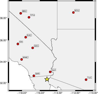
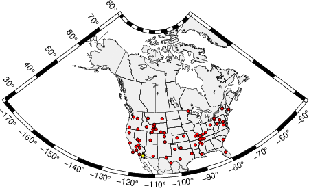
The focal mechanism was determined using broadband seismic waveforms. The location of the event (star) and the stations used for (red) the waveform inversion are shown in the next figure.
|
|
|
The program wvfgrd96 was used with good traces observed at short distance to determine the focal mechanism, depth and seismic moment. This technique requires a high quality signal and well determined velocity model for the Green's functions. To the extent that these are the quality data, this type of mechanism should be preferred over the radiation pattern technique which requires the separate step of defining the pressure and tension quadrants and the correct strike.
The observed and predicted traces are filtered using the following gsac commands:
cut o DIST/3.3 -30 o DIST/3.3 +90
rtr
taper w 0.1
hp c 0.03 n 3
lp c 0.05 n 3
The results of this grid search are as follow:
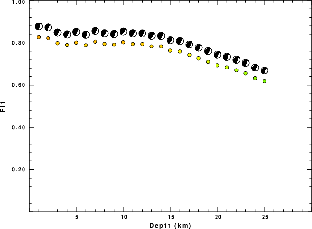
           DEPTH  STK   DIP  RAKE   MW    FIT
WVFGRD96    1.0   215    40   -85   4.98 0.2309
WVFGRD96    2.0   210    40   -95   5.06 0.2661
WVFGRD96    3.0    40    55   -80   5.11 0.2465
WVFGRD96    4.0    40    55   -80   5.13 0.2135
WVFGRD96    5.0   240    30   -40   5.11 0.1988
WVFGRD96    6.0   245    30   -35   5.10 0.1997
WVFGRD96    7.0   250    25   -30   5.09 0.2056
WVFGRD96    8.0   245    25   -35   5.16 0.2165
WVFGRD96    9.0   250    20   -30   5.16 0.2257
WVFGRD96   10.0   260    20   -15   5.15 0.2342
WVFGRD96   11.0   260    20   -15   5.15 0.2411
WVFGRD96   12.0   265    20   -10   5.15 0.2471
WVFGRD96   13.0   270    20    -5   5.15 0.2515
WVFGRD96   14.0   275    20     0   5.16 0.2549
WVFGRD96   15.0   280    20     5   5.16 0.2571
WVFGRD96   16.0   280    20     5   5.17 0.2585
WVFGRD96   17.0   290    20    15   5.17 0.2592
WVFGRD96   18.0   295    20    20   5.18 0.2592
WVFGRD96   19.0   185    80    65   5.20 0.2612
WVFGRD96   20.0   185    80    65   5.21 0.2620
WVFGRD96   21.0   185    80    65   5.23 0.2614
WVFGRD96   22.0   185    80    65   5.23 0.2607
WVFGRD96   23.0   185    80    65   5.24 0.2593
WVFGRD96   24.0   185    80    65   5.24 0.2574
WVFGRD96   25.0   190    75    65   5.25 0.2552
WVFGRD96   26.0   200    70    70   5.25 0.2536
WVFGRD96   27.0   200    70    70   5.25 0.2524
WVFGRD96   28.0   200    65    70   5.26 0.2511
WVFGRD96   29.0   200    65    70   5.26 0.2498
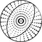
The best solution is
WVFGRD96 2.0 210 40 -95 5.06 0.2661
The mechanism corresponding to the best fit is
|
|
|
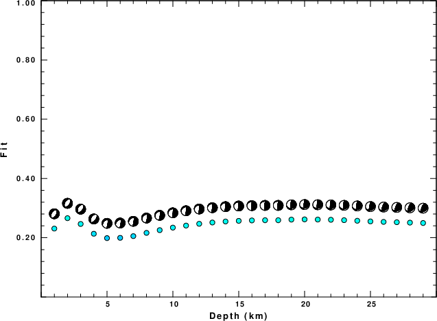
The best fit as a function of depth is given in the following figure:
|
|
|
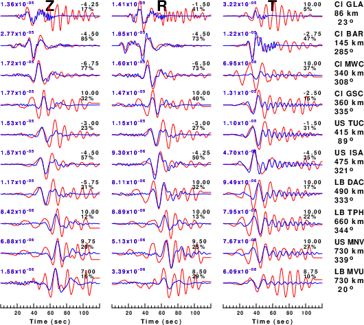
The comparison of the observed and predicted waveforms is given in the next figure. The red traces are the observed and the blue are the predicted. Each observed-predicted component is plotted to the same scale and peak amplitudes are indicated by the numbers to the left of each trace. A pair of numbers is given in black at the right of each predicted traces. The upper number it the time shift required for maximum correlation between the observed and predicted traces. This time shift is required because the synthetics are not computed at exactly the same distance as the observed, the velocity model used in the predictions may not be perfect and the epicentral parameters may be be off. A positive time shift indicates that the prediction is too fast and should be delayed to match the observed trace (shift to the right in this figure). A negative value indicates that the prediction is too slow. The lower number gives the percentage of variance reduction to characterize the individual goodness of fit (100% indicates a perfect fit).
The bandpass filter used in the processing and for the display was
cut o DIST/3.3 -30 o DIST/3.3 +90
rtr
taper w 0.1
hp c 0.03 n 3
lp c 0.05 n 3
|
| Figure 3. Waveform comparison for selected depth. Red: observed; Blue - predicted. The time shift with respect to the model prediction is indicated. The percent of fit is also indicated. The time scale is relative to the first trace sample. |
|
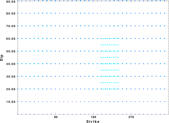
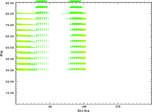
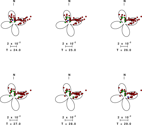
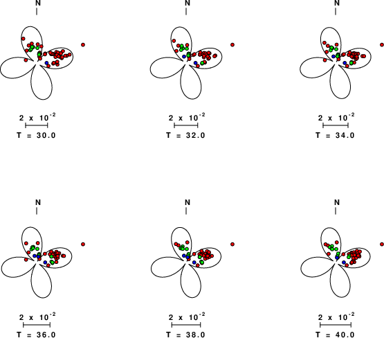
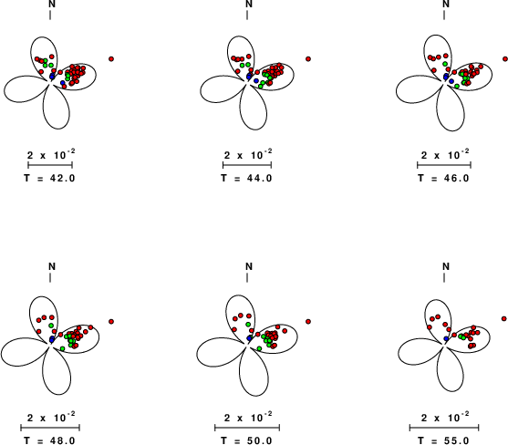
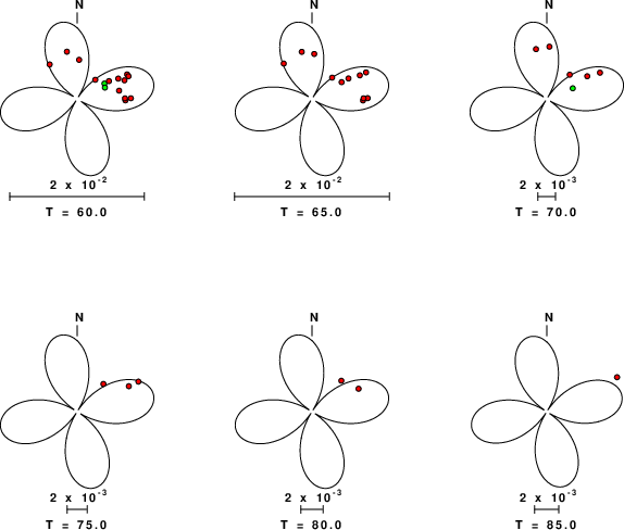
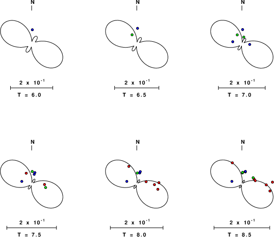
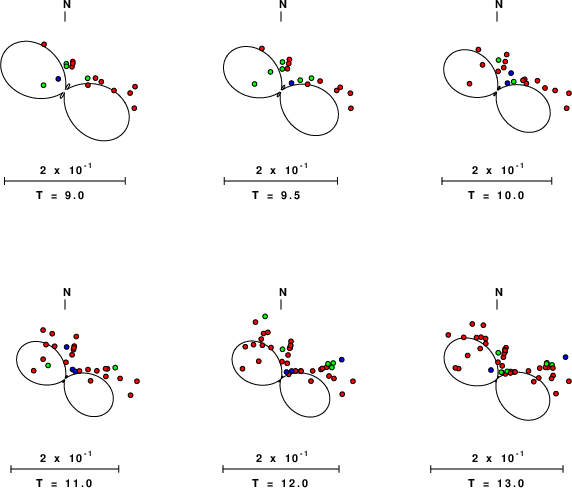
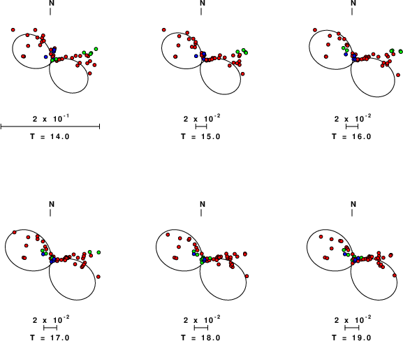
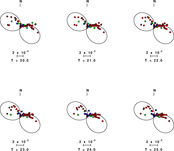
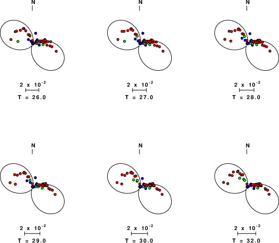
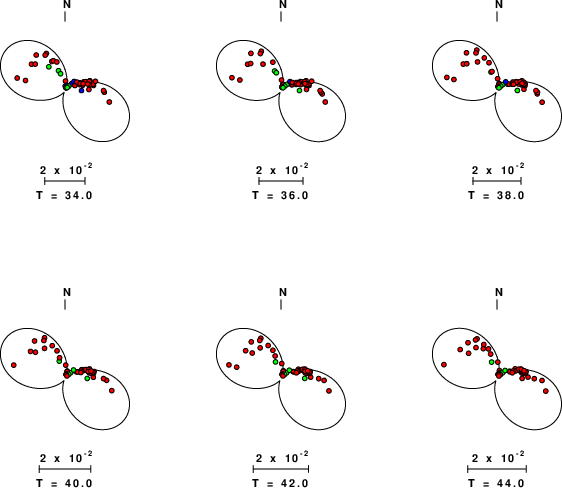
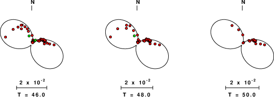
| Focal mechanism sensitivity at the preferred depth. The red color indicates a very good fit to the waveforms. Each solution is plotted as a vector at a given value of strike and dip with the angle of the vector representing the rake angle, measured, with respect to the upward vertical (N) in the figure. |
A check on the assumed source location is possible by looking at the time shifts between the observed and predicted traces. The time shifts for waveform matching arise for several reasons:
Time_shift = A + B cos Azimuth + C Sin Azimuth
The time shifts for this inversion lead to the next figure:
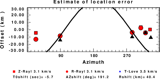
The derived shift in origin time and epicentral coordinates are given at the bottom of the figure.
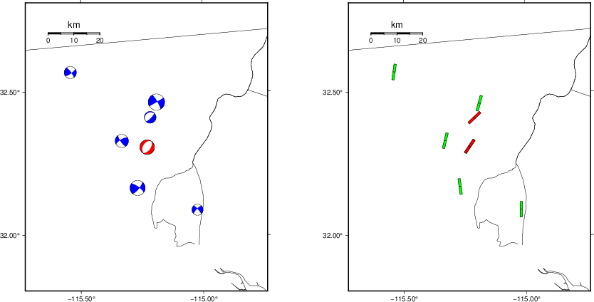
The following figure shows the stations used in the grid search for the best focal mechanism to fit the surface-wave spectral amplitudes of the Love and Rayleigh waves.
|
|
|
The surface-wave determined focal mechanism is shown here.
  NODAL PLANES


  STK=      10.00
  DIP=      54.99
 RAKE=    -120.00

             OR

  STK=     235.18
  DIP=      44.82
 RAKE=     -54.48


DEPTH = 1.0 km

Mw = 5.29
Best Fit 0.8217 - P-T axis plot gives solutions with FIT greater than FIT90
 |
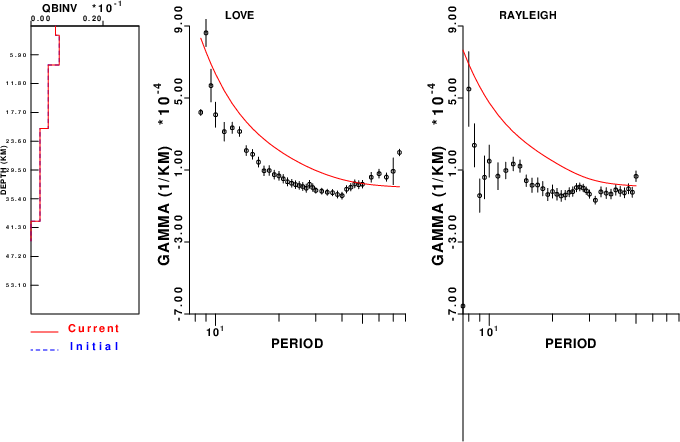
Surface wave analysis was performed using codes from Computer Programs in Seismology, specifically the multiple filter analysis program do_mft and the surface-wave radiation pattern search program srfgrd96.
Digital data were collected, instrument response removed and traces converted
to Z, R an T components. Multiple filter analysis was applied to the Z and T traces to obtain the Rayleigh- and Love-wave spectral amplitudes, respectively.
These were input to the search program which examined all depths between 1 and 25 km
and all possible mechanisms.
|
|
|

|
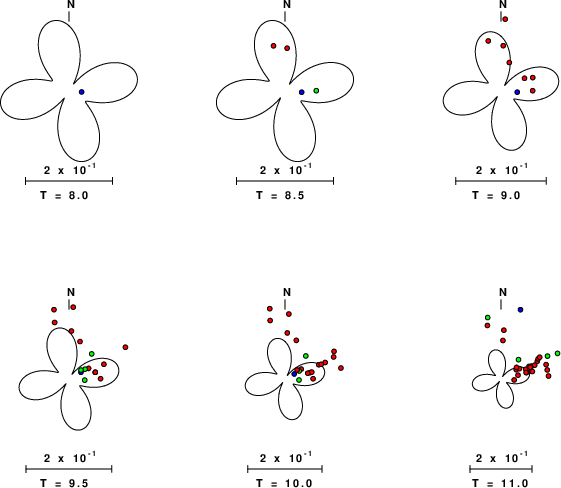
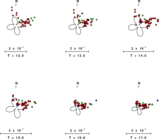
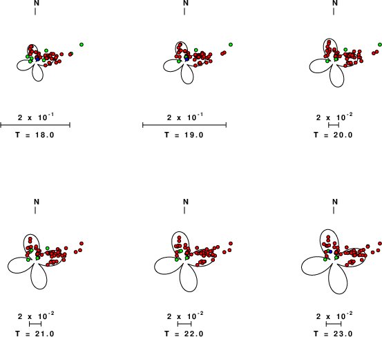
| Pressure-tension axis trends. Since the surface-wave spectra search does not distinguish between P and T axes and since there is a 180 ambiguity in strike, all possible P and T axes are plotted. First motion data and waveforms will be used to select the preferred mechanism. The purpose of this plot is to provide an idea of the possible range of solutions. The P and T-axes for all mechanisms with goodness of fit greater than 0.9 FITMAX (above) are plotted here. |
|
| Focal mechanism sensitivity at the preferred depth. The red color indicates a very good fit to the Love and Rayleigh wave radiation patterns. Each solution is plotted as a vector at a given value of strike and dip with the angle of the vector representing the rake angle, measured, with respect to the upward vertical (N) in the figure. Because of the symmetry of the spectral amplitude rediation patterns, only strikes from 0-180 degrees are sampled. |
|
|
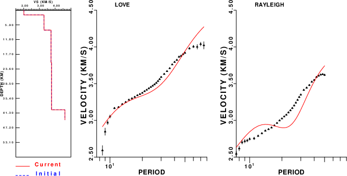
The WUS.model used for the waveform synthetic seismograms and for the surface wave eigenfunctions and dispersion is as follows (The format is in the model96 format of Computer Programs in Seismology).
MODEL.01
Model after     8 iterations
ISOTROPIC
KGS
FLAT EARTH
1-D
CONSTANT VELOCITY
LINE08
LINE09
LINE10
LINE11
      H(KM)   VP(KM/S)   VS(KM/S) RHO(GM/CC)         QP         QS       ETAP       ETAS      FREFP      FREFS
     1.9000     3.4065     2.0089     2.2150  0.302E-02  0.679E-02   0.00       0.00       1.00       1.00
     6.1000     5.5445     3.2953     2.6089  0.349E-02  0.784E-02   0.00       0.00       1.00       1.00
    13.0000     6.2708     3.7396     2.7812  0.212E-02  0.476E-02   0.00       0.00       1.00       1.00
    19.0000     6.4075     3.7680     2.8223  0.111E-02  0.249E-02   0.00       0.00       1.00       1.00
     0.0000     7.9000     4.6200     3.2760  0.164E-10  0.370E-10   0.00       0.00       1.00       1.00