The ANSS event ID is usp000ebfg and the event page is at https://earthquake.usgs.gov/earthquakes/eventpage/usp000ebfg/executive.
2006/03/05 10:42:16 64.911 -129.180 5.7 5.6 NWT, Canada
 USGS/SLU Moment Tensor Solution
 ENS  2006/03/05 10:42:16:0  64.91 -129.18   5.7 5.6 NWT, Canada

 Stations used:
   AK.BESE AK.BMR AK.BPAW AK.COLD AK.DCPH AK.DOT AK.EYAK
   AK.HARP AK.KTH AK.MCK AK.PAX AK.PNL AK.TRF AT.PMR AT.SIT
   AT.SKAG CN.DAWY CN.FNBB CN.GALN CN.INK CN.LUPN CN.MLON
   CN.WHY

 Filtering commands used:
   cut o DIST/3.3 -40 o DIST/3.3 +50
   rtr
   taper w 0.1
   hp c 0.03 n 3
   lp c 0.06 n 3

 Best Fitting Double Couple
  Mo = 1.48e+24 dyne-cm
  Mw = 5.38
  Z  = 2 km
  Plane   Strike  Dip  Rake
   NP1      288    45    85
   NP2      115    45    95
  Principal Axes:
   Axis    Value   Plunge  Azimuth
    T   1.48e+24     86     113
    N   0.00e+00      4     291
    P  -1.48e+24      0      21

 Moment Tensor: (dyne-cm)
    Component   Value
       Mxx    -1.28e+24
       Mxy    -5.06e+23
       Mxz    -3.85e+22
       Myy    -1.93e+23
       Myz     8.26e+22
       Mzz     1.47e+24


                     ------------ P
                 ----------------   ---
              ----------------------------
             ------------------------------
           ----------------------------------
          ----###################-------------
         --##########################----------
        -###############################--------
        --################################------
       ---#################################------
       ----##################   #############----
       -----################# T ##############---
       -------###############   ###############--
        -------################################-
        ---------###############################
         -----------###########################
          -------------######################-
           -----------------############-----
             ------------------------------
              ----------------------------
                 ----------------------
                     --------------


 Global CMT Convention Moment Tensor:
      R          T          P
  1.47e+24  -3.85e+22  -8.26e+22
 -3.85e+22  -1.28e+24   5.06e+23
 -8.26e+22   5.06e+23  -1.93e+23


Details of the solution is found at

http://www.eas.slu.edu/eqc/eqc_mt/MECH.NA/20060305104216/index.html
|
      STK = 115
      DIP = 45
     RAKE = 95
       MW = 5.38
       HS = 2.0
The NDK file is 20060305104216.ndk The waveform inversion is preferred.
The following compares this source inversion to those provided by others. The purpose is to look for major differences and also to note slight differences that might be inherent to the processing procedure. For completeness the USGS/SLU solution is repeated from above.
 USGS/SLU Moment Tensor Solution
 ENS  2006/03/05 10:42:16:0  64.91 -129.18   5.7 5.6 NWT, Canada

 Stations used:
   AK.BESE AK.BMR AK.BPAW AK.COLD AK.DCPH AK.DOT AK.EYAK
   AK.HARP AK.KTH AK.MCK AK.PAX AK.PNL AK.TRF AT.PMR AT.SIT
   AT.SKAG CN.DAWY CN.FNBB CN.GALN CN.INK CN.LUPN CN.MLON
   CN.WHY

 Filtering commands used:
   cut o DIST/3.3 -40 o DIST/3.3 +50
   rtr
   taper w 0.1
   hp c 0.03 n 3
   lp c 0.06 n 3

 Best Fitting Double Couple
  Mo = 1.48e+24 dyne-cm
  Mw = 5.38
  Z  = 2 km
  Plane   Strike  Dip  Rake
   NP1      288    45    85
   NP2      115    45    95
  Principal Axes:
   Axis    Value   Plunge  Azimuth
    T   1.48e+24     86     113
    N   0.00e+00      4     291
    P  -1.48e+24      0      21

 Moment Tensor: (dyne-cm)
    Component   Value
       Mxx    -1.28e+24
       Mxy    -5.06e+23
       Mxz    -3.85e+22
       Myy    -1.93e+23
       Myz     8.26e+22
       Mzz     1.47e+24


                     ------------ P
                 ----------------   ---
              ----------------------------
             ------------------------------
           ----------------------------------
          ----###################-------------
         --##########################----------
        -###############################--------
        --################################------
       ---#################################------
       ----##################   #############----
       -----################# T ##############---
       -------###############   ###############--
        -------################################-
        ---------###############################
         -----------###########################
          -------------######################-
           -----------------############-----
             ------------------------------
              ----------------------------
                 ----------------------
                     --------------


 Global CMT Convention Moment Tensor:
      R          T          P
  1.47e+24  -3.85e+22  -8.26e+22
 -3.85e+22  -1.28e+24   5.06e+23
 -8.26e+22   5.06e+23  -1.93e+23


Details of the solution is found at

http://www.eas.slu.edu/eqc/eqc_mt/MECH.NA/20060305104216/index.html
|
March 5, 2006, NORTHWEST TERRITORIES, CANADA, MW=5.5

Natasha Maternovskaya

CENTROID, MOMENT TENSOR SOLUTION
HARVARD EVENT-FILE NAME C030506B
DATA USED: GSN
L.P. BODY WAVES: 61S,123C, T= 40
SURFACE WAVES:   81S,181C, T= 50
CENTROID LOCATION:
ORIGIN TIME       10:42:19.6 0.1
LAT 65.05N 0.01;LON 129.19W 0.03
DEP  12.0 FIX;HALF-DURATION  1.3
MOMENT TENSOR; SCALE 10**24 D-CM
  MRR= 1.88 0.03; MTT=-1.68 0.02
  MPP=-0.21 0.02; MRT= 0.13 0.07
  MRP=-0.13 0.07; MTP= 0.70 0.02
 PRINCIPAL AXES:
 1.(T) VAL=  1.89;PLG=87;AZM= 64
 2.(N)       0.07;     2;    292
 3.(P)      -1.96;     2;    202
BEST DOUBLE COUPLE:M0=1.9*10**24
 NP1:STRIKE=289;DIP=43;SLIP=  87
 NP2:STRIKE=114;DIP=48;SLIP=  93

            -----------
        -------------------
      -----------------------
    ---------------------------
   ---################----------
  -######################--------
  -#########################-----
 --##############   ##########----
 ---############# T ###########---
 ----############   ############--
 ------##########################-
  -------########################
  ----------#####################
   ------------###############--
    ---------------------------
      -----------------------
        --   --------------
           P ----------
|
|
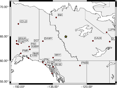
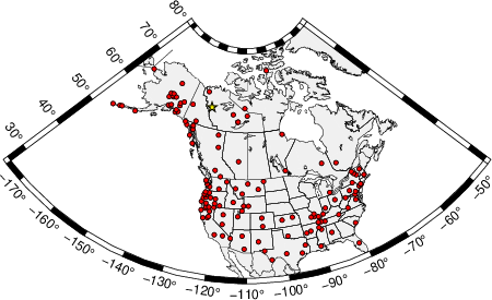
The focal mechanism was determined using broadband seismic waveforms. The location of the event (star) and the stations used for (red) the waveform inversion are shown in the next figure.
|
|
|
The program wvfgrd96 was used with good traces observed at short distance to determine the focal mechanism, depth and seismic moment. This technique requires a high quality signal and well determined velocity model for the Green's functions. To the extent that these are the quality data, this type of mechanism should be preferred over the radiation pattern technique which requires the separate step of defining the pressure and tension quadrants and the correct strike.
The observed and predicted traces are filtered using the following gsac commands:
cut o DIST/3.3 -40 o DIST/3.3 +50
rtr
taper w 0.1
hp c 0.03 n 3
lp c 0.06 n 3
The results of this grid search are as follow:
           DEPTH  STK   DIP  RAKE   MW    FIT
WVFGRD96    1.0    95    50    65   5.32 0.5277
WVFGRD96    2.0   115    45    95   5.38 0.5608
WVFGRD96    3.0   115    45    95   5.43 0.5402
WVFGRD96    4.0   115    60    95   5.45 0.4805
WVFGRD96    5.0   115    60    95   5.44 0.4526
WVFGRD96    6.0   110    65    90   5.42 0.4418
WVFGRD96    7.0   295    25    95   5.41 0.4393
WVFGRD96    8.0   295    30    95   5.41 0.4400
WVFGRD96    9.0   235    55   -30   5.34 0.4462
WVFGRD96   10.0   105    65    80   5.42 0.4497
WVFGRD96   11.0   235    60   -35   5.37 0.4613
WVFGRD96   12.0   235    60   -35   5.38 0.4720
WVFGRD96   13.0   235    60   -40   5.39 0.4819
WVFGRD96   14.0   235    60   -40   5.39 0.4901
WVFGRD96   15.0   235    60   -40   5.40 0.4965
WVFGRD96   16.0   235    60   -40   5.41 0.5014
WVFGRD96   17.0   235    60   -40   5.41 0.5050
WVFGRD96   18.0   235    60   -40   5.42 0.5079
WVFGRD96   19.0   235    60   -40   5.42 0.5104
WVFGRD96   20.0   235    60   -40   5.44 0.5051
WVFGRD96   21.0   235    60   -40   5.45 0.5041
WVFGRD96   22.0   235    60   -40   5.45 0.5021
WVFGRD96   23.0   235    65   -40   5.46 0.4994
WVFGRD96   24.0   135    40   -55   5.47 0.4961
WVFGRD96   25.0   135    40   -55   5.47 0.4959
WVFGRD96   26.0   135    40   -55   5.48 0.4949
WVFGRD96   27.0   135    40   -55   5.48 0.4934
WVFGRD96   28.0   135    40   -55   5.49 0.4917
WVFGRD96   29.0   135    40   -55   5.49 0.4897
The best solution is
WVFGRD96 2.0 115 45 95 5.38 0.5608
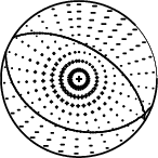
The mechanism corresponding to the best fit is
|
|
|
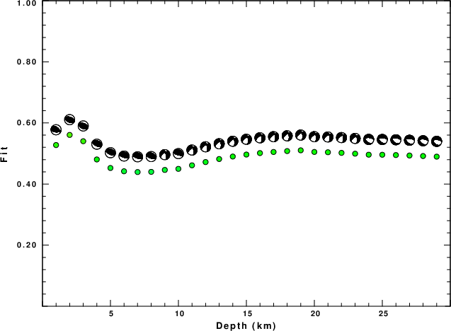
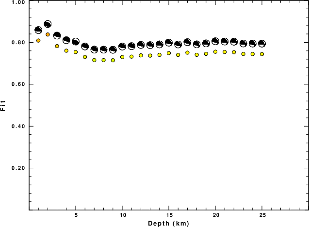
The best fit as a function of depth is given in the following figure:
|
|
|
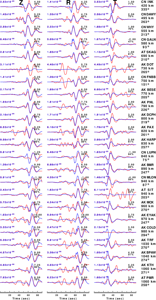
The comparison of the observed and predicted waveforms is given in the next figure. The red traces are the observed and the blue are the predicted. Each observed-predicted component is plotted to the same scale and peak amplitudes are indicated by the numbers to the left of each trace. A pair of numbers is given in black at the right of each predicted traces. The upper number it the time shift required for maximum correlation between the observed and predicted traces. This time shift is required because the synthetics are not computed at exactly the same distance as the observed, the velocity model used in the predictions may not be perfect and the epicentral parameters may be be off. A positive time shift indicates that the prediction is too fast and should be delayed to match the observed trace (shift to the right in this figure). A negative value indicates that the prediction is too slow. The lower number gives the percentage of variance reduction to characterize the individual goodness of fit (100% indicates a perfect fit).
The bandpass filter used in the processing and for the display was
cut o DIST/3.3 -40 o DIST/3.3 +50
rtr
taper w 0.1
hp c 0.03 n 3
lp c 0.06 n 3
|
| Figure 3. Waveform comparison for selected depth. Red: observed; Blue - predicted. The time shift with respect to the model prediction is indicated. The percent of fit is also indicated. The time scale is relative to the first trace sample. |
|
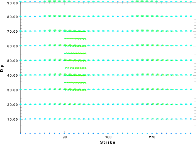
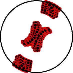
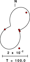
| Focal mechanism sensitivity at the preferred depth. The red color indicates a very good fit to the waveforms. Each solution is plotted as a vector at a given value of strike and dip with the angle of the vector representing the rake angle, measured, with respect to the upward vertical (N) in the figure. |
A check on the assumed source location is possible by looking at the time shifts between the observed and predicted traces. The time shifts for waveform matching arise for several reasons:
Time_shift = A + B cos Azimuth + C Sin Azimuth
The time shifts for this inversion lead to the next figure:
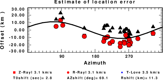
The derived shift in origin time and epicentral coordinates are given at the bottom of the figure.
The following figure shows the stations used in the grid search for the best focal mechanism to fit the surface-wave spectral amplitudes of the Love and Rayleigh waves.
|
|
|
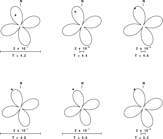
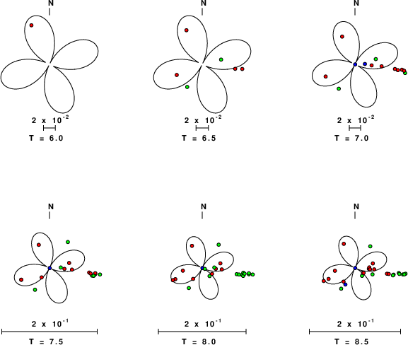
The surface-wave determined focal mechanism is shown here.
  NODAL PLANES


  STK=     302.15
  DIP=      55.61
 RAKE=      96.93

             OR

  STK=     110.00
  DIP=      35.00
 RAKE=      80.00


DEPTH = 2.0 km

Mw = 5.46
Best Fit 0.8378 - P-T axis plot gives solutions with FIT greater than FIT90
 |
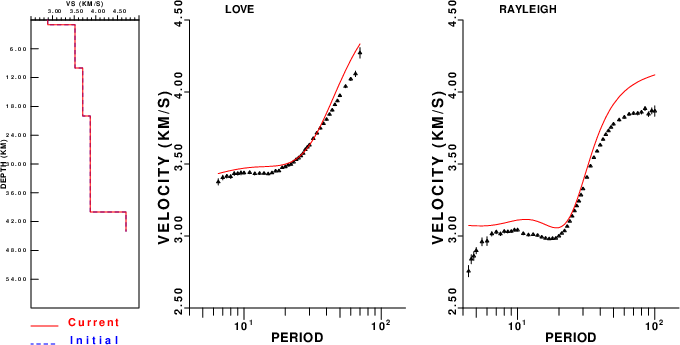
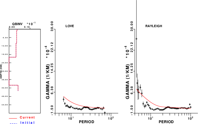
Surface wave analysis was performed using codes from Computer Programs in Seismology, specifically the multiple filter analysis program do_mft and the surface-wave radiation pattern search program srfgrd96.
Digital data were collected, instrument response removed and traces converted
to Z, R an T components. Multiple filter analysis was applied to the Z and T traces to obtain the Rayleigh- and Love-wave spectral amplitudes, respectively.
These were input to the search program which examined all depths between 1 and 25 km
and all possible mechanisms.
|
|
|
|
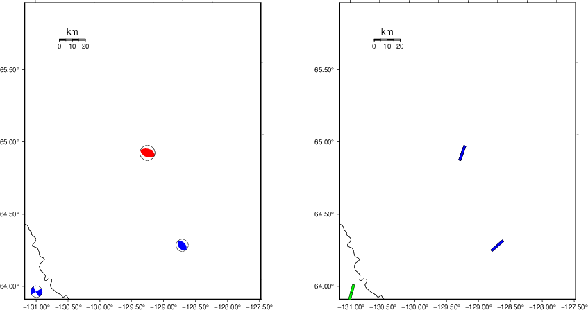
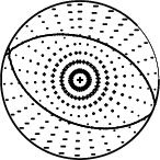
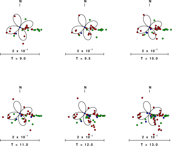
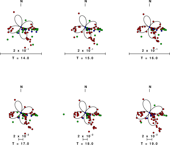
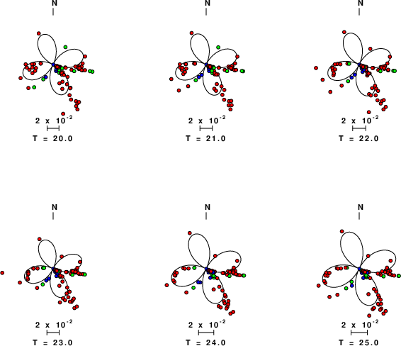
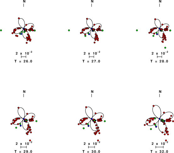
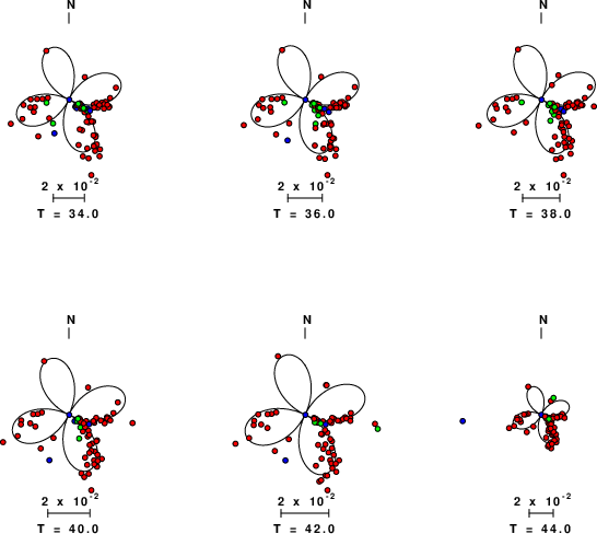
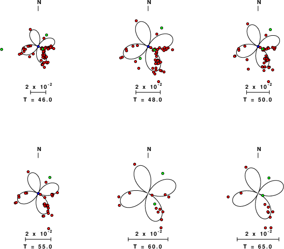
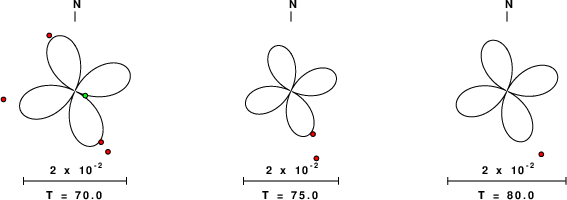
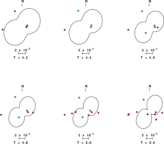
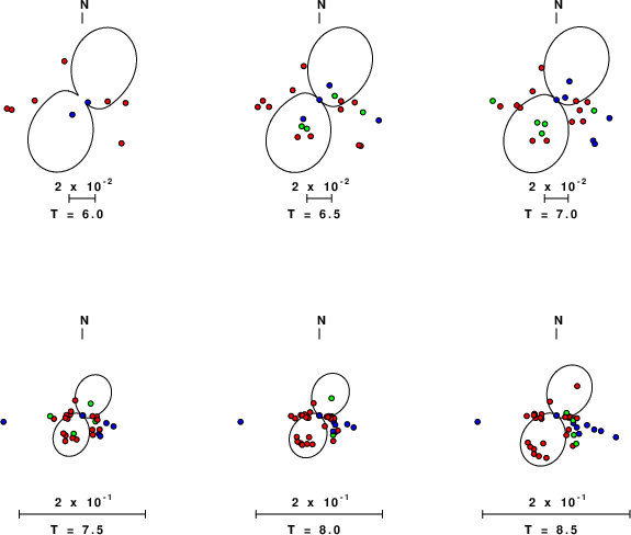
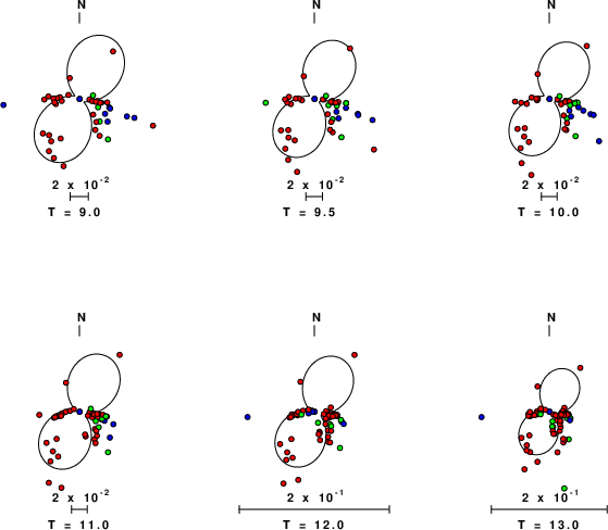
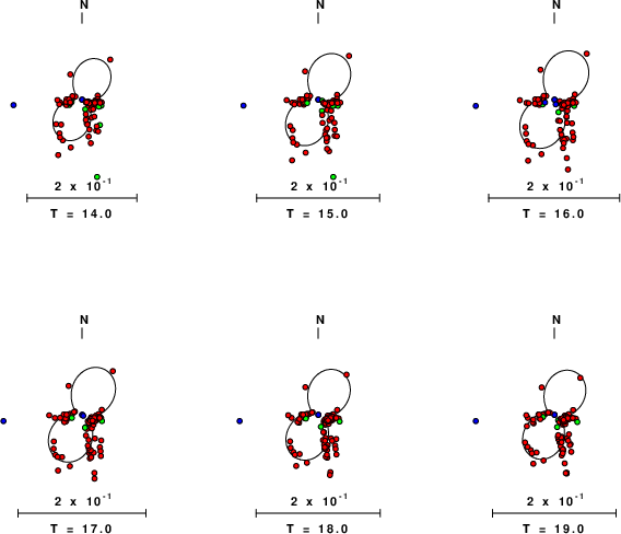
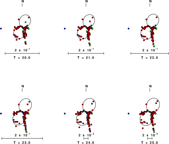
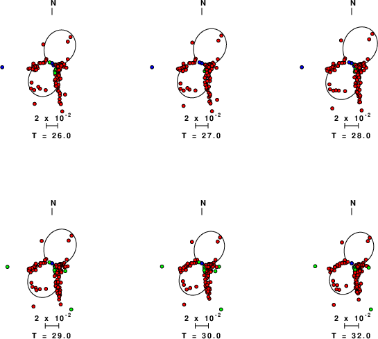
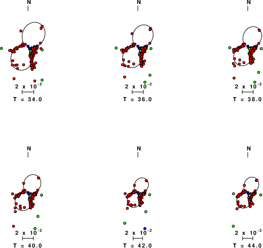
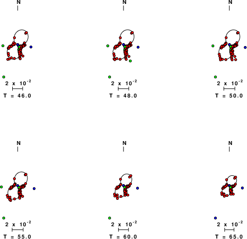
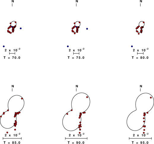
| Pressure-tension axis trends. Since the surface-wave spectra search does not distinguish between P and T axes and since there is a 180 ambiguity in strike, all possible P and T axes are plotted. First motion data and waveforms will be used to select the preferred mechanism. The purpose of this plot is to provide an idea of the possible range of solutions. The P and T-axes for all mechanisms with goodness of fit greater than 0.9 FITMAX (above) are plotted here. |
|
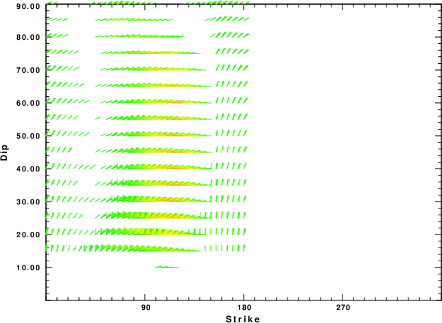
| Focal mechanism sensitivity at the preferred depth. The red color indicates a very good fit to the Love and Rayleigh wave radiation patterns. Each solution is plotted as a vector at a given value of strike and dip with the angle of the vector representing the rake angle, measured, with respect to the upward vertical (N) in the figure. Because of the symmetry of the spectral amplitude rediation patterns, only strikes from 0-180 degrees are sampled. |
|
|
The CUS.model used for the waveform synthetic seismograms and for the surface wave eigenfunctions and dispersion is as follows (The format is in the model96 format of Computer Programs in Seismology).
MODEL.01
CUS Model with Q from simple gamma values
ISOTROPIC
KGS
FLAT EARTH
1-D
CONSTANT VELOCITY
LINE08
LINE09
LINE10
LINE11
  H(KM) VP(KM/S) VS(KM/S) RHO(GM/CC)   QP   QS  ETAP  ETAS  FREFP  FREFS
  1.0000  5.0000  2.8900  2.5000 0.172E-02 0.387E-02 0.00  0.00  1.00  1.00
  9.0000  6.1000  3.5200  2.7300 0.160E-02 0.363E-02 0.00  0.00  1.00  1.00
 10.0000  6.4000  3.7000  2.8200 0.149E-02 0.336E-02 0.00  0.00  1.00  1.00
 20.0000  6.7000  3.8700  2.9020 0.000E-04 0.000E-04 0.00  0.00  1.00  1.00
  0.0000  8.1500  4.7000  3.3640 0.194E-02 0.431E-02 0.00  0.00  1.00  1.00