The ANSS event ID is usp000e365 and the event page is at https://earthquake.usgs.gov/earthquakes/eventpage/usp000e365/executive.
2005/10/31 00:23:30 44.874 -113.399 5.0 4.5 Montana
 USGS/SLU Moment Tensor Solution
 ENS  2005/10/31 00:23:30:0  44.87 -113.40   5.0 4.5 Montana

 Stations used:
   US.AHID US.BW06 US.HAWA US.HLID US.HWUT US.LAO US.LKWY
   US.MSO US.REDW

 Filtering commands used:
   cut o DIST/3.3 -40 o DIST/3.3 +50
   rtr
   taper w 0.1
   hp c 0.03 n 3
   lp c 0.06 n 3

 Best Fitting Double Couple
  Mo = 5.56e+22 dyne-cm
  Mw = 4.43
  Z  = 15 km
  Plane   Strike  Dip  Rake
   NP1      303    82   -114
   NP2      195    25   -20
  Principal Axes:
   Axis    Value   Plunge  Azimuth
    T   5.56e+22     33      53
    N   0.00e+00     23     307
    P  -5.56e+22     48     188

 Moment Tensor: (dyne-cm)
    Component   Value
       Mxx    -1.01e+22
       Mxy     1.55e+22
       Mxz     4.26e+22
       Myy     2.46e+22
       Myz     2.41e+22
       Mzz    -1.46e+22


                     -------#######
                 ------################
              ------######################
             -----#########################
           ------############################
          ####-#######################   #####
         #####----#################### T ######
        ######-------#################   #######
        #####------------#######################
       #####----------------#####################
       #####------------------###################
       #####---------------------################
       #####------------------------#############
        ####--------------------------##########
        #####---------------------------########
         ####------------   --------------#####
          ####----------- P ----------------##
           ####----------   -----------------
             ###---------------------------
              ###-------------------------
                 ##--------------------
                     #-------------


 Global CMT Convention Moment Tensor:
      R          T          P
 -1.46e+22   4.26e+22  -2.41e+22
  4.26e+22  -1.01e+22  -1.55e+22
 -2.41e+22  -1.55e+22   2.46e+22


Details of the solution is found at

http://www.eas.slu.edu/eqc/eqc_mt/MECH.NA/20051031002330/index.html
|
      STK = 195
      DIP = 25
     RAKE = -20
       MW = 4.43
       HS = 15.0
The NDK file is 20051031002330.ndk The waveform inversion is preferred.
The following compares this source inversion to those provided by others. The purpose is to look for major differences and also to note slight differences that might be inherent to the processing procedure. For completeness the USGS/SLU solution is repeated from above.
 USGS/SLU Moment Tensor Solution
 ENS  2005/10/31 00:23:30:0  44.87 -113.40   5.0 4.5 Montana

 Stations used:
   US.AHID US.BW06 US.HAWA US.HLID US.HWUT US.LAO US.LKWY
   US.MSO US.REDW

 Filtering commands used:
   cut o DIST/3.3 -40 o DIST/3.3 +50
   rtr
   taper w 0.1
   hp c 0.03 n 3
   lp c 0.06 n 3

 Best Fitting Double Couple
  Mo = 5.56e+22 dyne-cm
  Mw = 4.43
  Z  = 15 km
  Plane   Strike  Dip  Rake
   NP1      303    82   -114
   NP2      195    25   -20
  Principal Axes:
   Axis    Value   Plunge  Azimuth
    T   5.56e+22     33      53
    N   0.00e+00     23     307
    P  -5.56e+22     48     188

 Moment Tensor: (dyne-cm)
    Component   Value
       Mxx    -1.01e+22
       Mxy     1.55e+22
       Mxz     4.26e+22
       Myy     2.46e+22
       Myz     2.41e+22
       Mzz    -1.46e+22


                     -------#######
                 ------################
              ------######################
             -----#########################
           ------############################
          ####-#######################   #####
         #####----#################### T ######
        ######-------#################   #######
        #####------------#######################
       #####----------------#####################
       #####------------------###################
       #####---------------------################
       #####------------------------#############
        ####--------------------------##########
        #####---------------------------########
         ####------------   --------------#####
          ####----------- P ----------------##
           ####----------   -----------------
             ###---------------------------
              ###-------------------------
                 ##--------------------
                     #-------------


 Global CMT Convention Moment Tensor:
      R          T          P
 -1.46e+22   4.26e+22  -2.41e+22
  4.26e+22  -1.01e+22  -1.55e+22
 -2.41e+22  -1.55e+22   2.46e+22


Details of the solution is found at

http://www.eas.slu.edu/eqc/eqc_mt/MECH.NA/20051031002330/index.html
|
Harvard CMT Event name: 103105B

Region name: WESTERN MONTANA
Date (y/m/d): 2005/10/31

Information on data used in inversion

Wave    nsta  nrec  cutoff
Body       0     0   0
Mantle    26    36   40

Timing and location information

         hr  min   sec       lat     lon    depth   mb   Ms
PDE       0   23  30.00     44.90  -113.45    5.0  4.5  4.5
CMT       0   23  34.90     44.83  -113.30   13.4
Error              0.50      0.03     0.05    3.0
Assumed half duration:  0.4


Mechanism information

Exponent for moment tensor:  22    units: dyne-cm
         Mrr     Mtt     Mpp     Mrt     Mrp     Mtp
CMT    -4.030   0.340   3.690   5.250  -3.300  -3.050
Error   0.790   0.400   0.530   1.510   1.100   0.320

Mw = 4.5   Scalar Moment = 7.91e+22
Fault plane:  strike=176    dip=25   slip=-44
Fault plane:  strike=307    dip=73   slip=-108
Eigenvector:  eigenvalue:  8.17   plunge: 26   azimuth:  51
Eigenvector:  eigenvalue: -0.53   plunge: 18   azimuth: 312
Eigenvector:  eigenvalue: -7.65   plunge: 58   azimuth: 192
|
|
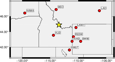
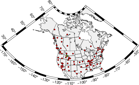
The focal mechanism was determined using broadband seismic waveforms. The location of the event (star) and the stations used for (red) the waveform inversion are shown in the next figure.
|
|
|
The program wvfgrd96 was used with good traces observed at short distance to determine the focal mechanism, depth and seismic moment. This technique requires a high quality signal and well determined velocity model for the Green's functions. To the extent that these are the quality data, this type of mechanism should be preferred over the radiation pattern technique which requires the separate step of defining the pressure and tension quadrants and the correct strike.
The observed and predicted traces are filtered using the following gsac commands:
cut o DIST/3.3 -40 o DIST/3.3 +50
rtr
taper w 0.1
hp c 0.03 n 3
lp c 0.06 n 3
The results of this grid search are as follow:
           DEPTH  STK   DIP  RAKE   MW    FIT
WVFGRD96    1.0   315    40   -90   4.21 0.4747
WVFGRD96    2.0   315    40   -90   4.28 0.5069
WVFGRD96    3.0   320    30   -80   4.33 0.4185
WVFGRD96    4.0   355    25   -35   4.34 0.4415
WVFGRD96    5.0     0    25   -30   4.33 0.4797
WVFGRD96    6.0   185    20   -25   4.34 0.5251
WVFGRD96    7.0   185    20   -30   4.34 0.5679
WVFGRD96    8.0   180    15   -35   4.42 0.5988
WVFGRD96    9.0   180    20   -35   4.42 0.6336
WVFGRD96   10.0   185    20   -30   4.42 0.6597
WVFGRD96   11.0   180    20   -40   4.43 0.6786
WVFGRD96   12.0   180    20   -40   4.43 0.6927
WVFGRD96   13.0   190    25   -25   4.43 0.7023
WVFGRD96   14.0   190    25   -25   4.43 0.7080
WVFGRD96   15.0   195    25   -20   4.43 0.7101
WVFGRD96   16.0   195    25   -20   4.44 0.7095
WVFGRD96   17.0   190    25   -30   4.45 0.7058
WVFGRD96   18.0   195    25   -25   4.45 0.7004
WVFGRD96   19.0   195    25   -25   4.46 0.6932
WVFGRD96   20.0   200    25   -15   4.46 0.6841
WVFGRD96   21.0   200    25   -20   4.48 0.6740
WVFGRD96   22.0   200    25   -20   4.48 0.6626
WVFGRD96   23.0   200    25   -20   4.49 0.6498
WVFGRD96   24.0   205    25   -10   4.49 0.6361
WVFGRD96   25.0   205    25   -15   4.50 0.6216
WVFGRD96   26.0   205    25   -15   4.51 0.6068
WVFGRD96   27.0   205    25   -15   4.51 0.5913
WVFGRD96   28.0   205    25   -15   4.52 0.5751
WVFGRD96   29.0   205    25   -15   4.52 0.5584
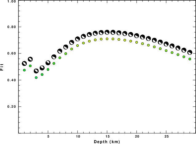
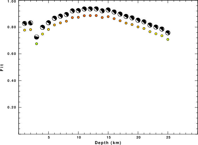
The best solution is
WVFGRD96 15.0 195 25 -20 4.43 0.7101
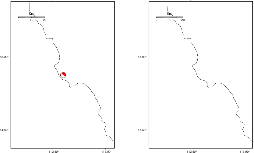
The mechanism corresponding to the best fit is
|
|
|
The best fit as a function of depth is given in the following figure:
|
|
|
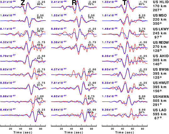
The comparison of the observed and predicted waveforms is given in the next figure. The red traces are the observed and the blue are the predicted. Each observed-predicted component is plotted to the same scale and peak amplitudes are indicated by the numbers to the left of each trace. A pair of numbers is given in black at the right of each predicted traces. The upper number it the time shift required for maximum correlation between the observed and predicted traces. This time shift is required because the synthetics are not computed at exactly the same distance as the observed, the velocity model used in the predictions may not be perfect and the epicentral parameters may be be off. A positive time shift indicates that the prediction is too fast and should be delayed to match the observed trace (shift to the right in this figure). A negative value indicates that the prediction is too slow. The lower number gives the percentage of variance reduction to characterize the individual goodness of fit (100% indicates a perfect fit).
The bandpass filter used in the processing and for the display was
cut o DIST/3.3 -40 o DIST/3.3 +50
rtr
taper w 0.1
hp c 0.03 n 3
lp c 0.06 n 3
|
| Figure 3. Waveform comparison for selected depth. Red: observed; Blue - predicted. The time shift with respect to the model prediction is indicated. The percent of fit is also indicated. The time scale is relative to the first trace sample. |
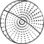
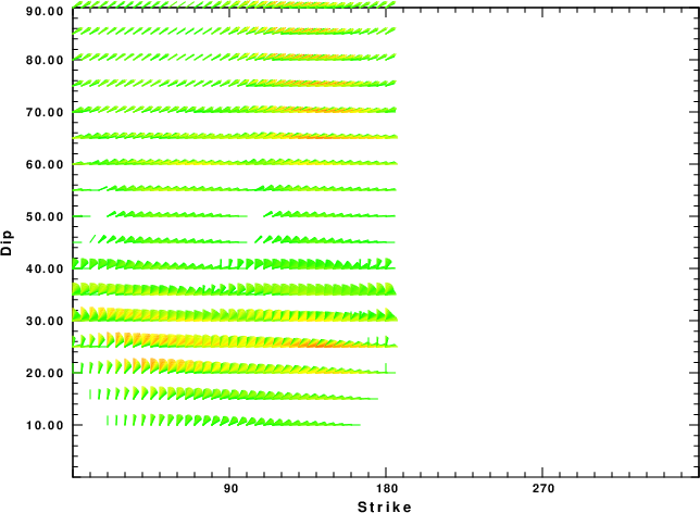
|
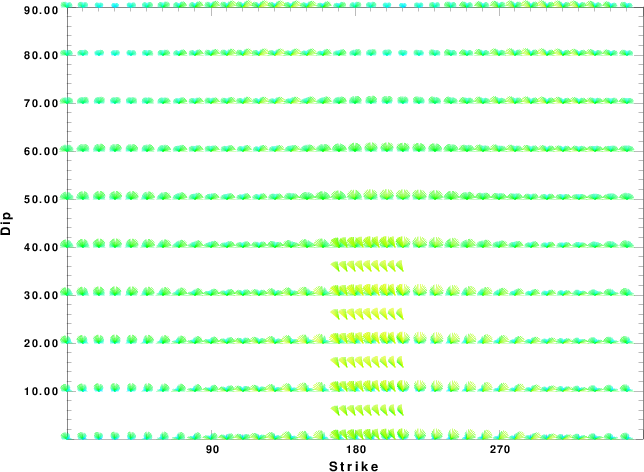
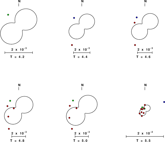
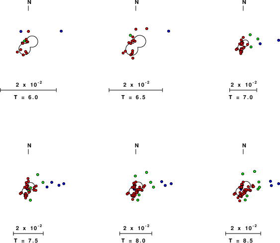
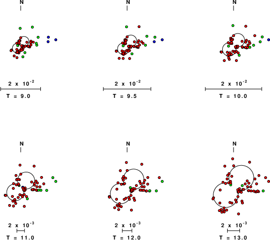
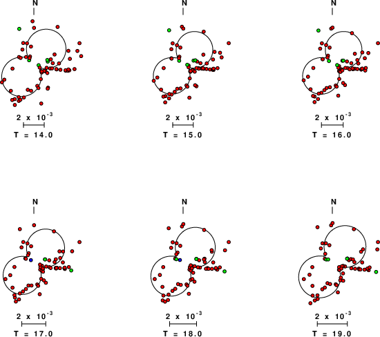
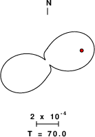
| Focal mechanism sensitivity at the preferred depth. The red color indicates a very good fit to the waveforms. Each solution is plotted as a vector at a given value of strike and dip with the angle of the vector representing the rake angle, measured, with respect to the upward vertical (N) in the figure. |
A check on the assumed source location is possible by looking at the time shifts between the observed and predicted traces. The time shifts for waveform matching arise for several reasons:
Time_shift = A + B cos Azimuth + C Sin Azimuth
The time shifts for this inversion lead to the next figure:
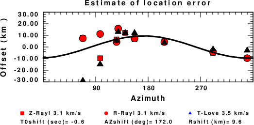
The derived shift in origin time and epicentral coordinates are given at the bottom of the figure.
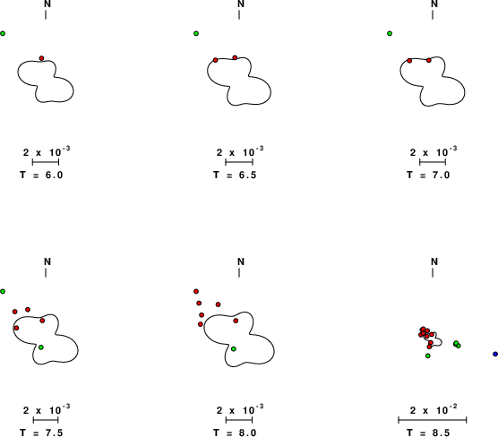
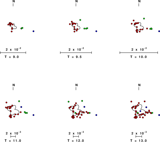
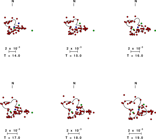
The following figure shows the stations used in the grid search for the best focal mechanism to fit the surface-wave spectral amplitudes of the Love and Rayleigh waves.
|
|
|
The surface-wave determined focal mechanism is shown here.
  NODAL PLANES


  STK=     314.98
  DIP=      74.99
 RAKE=    -105.00

             OR

  STK=     180.97
  DIP=      21.09
 RAKE=     -46.00


DEPTH = 13.0 km

Mw = 4.53
Best Fit 0.8862 - P-T axis plot gives solutions with FIT greater than FIT90
 |
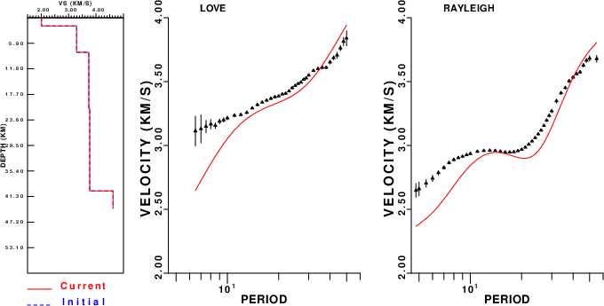
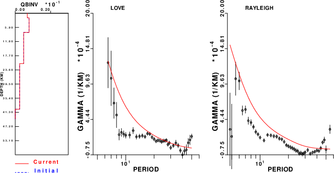
Surface wave analysis was performed using codes from Computer Programs in Seismology, specifically the multiple filter analysis program do_mft and the surface-wave radiation pattern search program srfgrd96.
Digital data were collected, instrument response removed and traces converted
to Z, R an T components. Multiple filter analysis was applied to the Z and T traces to obtain the Rayleigh- and Love-wave spectral amplitudes, respectively.
These were input to the search program which examined all depths between 1 and 25 km
and all possible mechanisms.
|
|
|

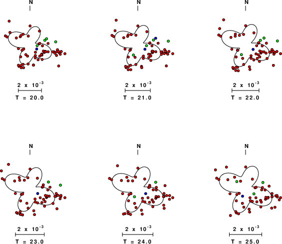
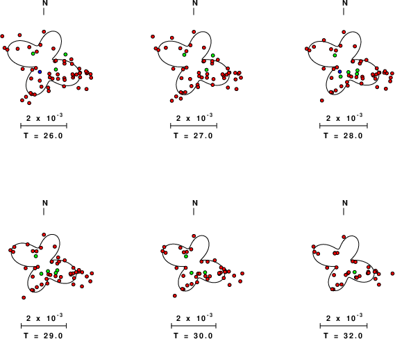
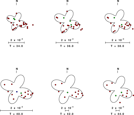
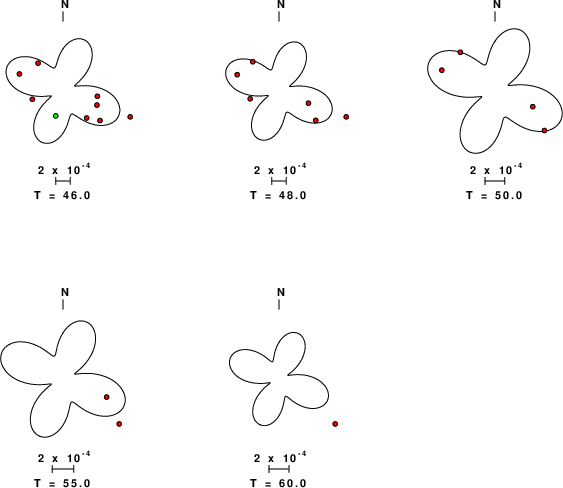
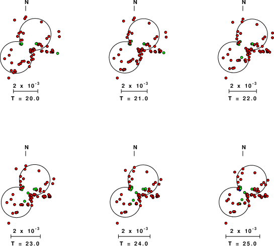
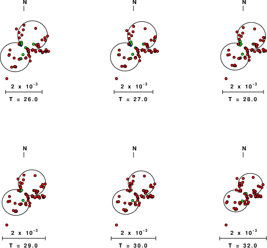
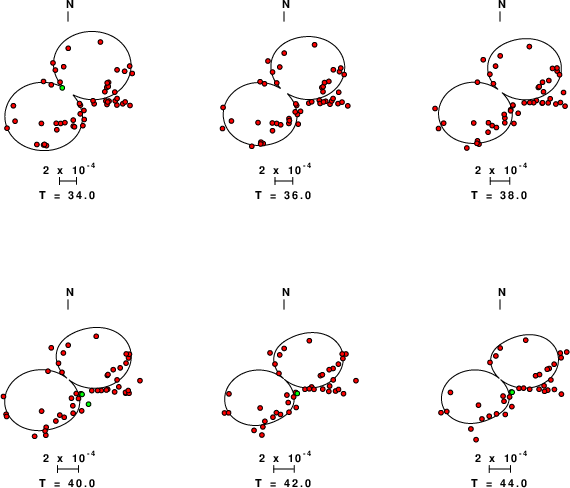
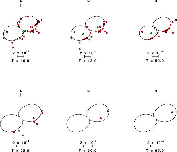
|
| Pressure-tension axis trends. Since the surface-wave spectra search does not distinguish between P and T axes and since there is a 180 ambiguity in strike, all possible P and T axes are plotted. First motion data and waveforms will be used to select the preferred mechanism. The purpose of this plot is to provide an idea of the possible range of solutions. The P and T-axes for all mechanisms with goodness of fit greater than 0.9 FITMAX (above) are plotted here. |
|
| Focal mechanism sensitivity at the preferred depth. The red color indicates a very good fit to the Love and Rayleigh wave radiation patterns. Each solution is plotted as a vector at a given value of strike and dip with the angle of the vector representing the rake angle, measured, with respect to the upward vertical (N) in the figure. Because of the symmetry of the spectral amplitude rediation patterns, only strikes from 0-180 degrees are sampled. |
|
|
The WUS.model used for the waveform synthetic seismograms and for the surface wave eigenfunctions and dispersion is as follows (The format is in the model96 format of Computer Programs in Seismology).
MODEL.01
Model after     8 iterations
ISOTROPIC
KGS
FLAT EARTH
1-D
CONSTANT VELOCITY
LINE08
LINE09
LINE10
LINE11
      H(KM)   VP(KM/S)   VS(KM/S) RHO(GM/CC)         QP         QS       ETAP       ETAS      FREFP      FREFS
     1.9000     3.4065     2.0089     2.2150  0.302E-02  0.679E-02   0.00       0.00       1.00       1.00
     6.1000     5.5445     3.2953     2.6089  0.349E-02  0.784E-02   0.00       0.00       1.00       1.00
    13.0000     6.2708     3.7396     2.7812  0.212E-02  0.476E-02   0.00       0.00       1.00       1.00
    19.0000     6.4075     3.7680     2.8223  0.111E-02  0.249E-02   0.00       0.00       1.00       1.00
     0.0000     7.9000     4.6200     3.2760  0.164E-10  0.370E-10   0.00       0.00       1.00       1.00